Tskit for population genetics#
Tskit, the tree sequence toolkit, brings the power of evolutionary trees to the field of population genetics. The succinct tree sequence format is designed to store DNA sequences jointly with their ancestral history (the “genetic genealogy” or ARG). Storing population genetic data in this form enables highly efficient computation and analysis.
The core tskit library provides methods for storing genetic data, a flexible analysis framework, and APIs to build your own efficient population genetic algorithms. Because of its speed and scalability, tskit is well-suited to interactive analysis of large genomic datasets.
Population genetic simulation#
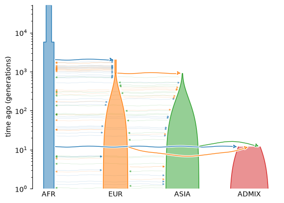
Several simulation tools output tree sequences. Below we use the standard library for population genetic simulation models (stdpopsim) to generate a model of Homo sapiens, in which African, Eurasian, and Asian populations combine to generate a mixed American population. We can use the demesdraw package to plot a schematic of the migrations and population size changes that define this model.
import stdpopsim
import demesdraw
from matplotlib import pyplot as plt

species = stdpopsim.get_species("HomSap")
model = species.get_demographic_model("AmericanAdmixture_4B18")

# Plot a schematic of the model
demesdraw.tubes(model.model.to_demes(), ax=plt.gca(), seed=1, log_time=True)
plt.show()
Genomic data in tree sequence format can be generated via the widely-used
msprime simulator. Here we simulate 1
megabase of genome sequence at the start of human chromosome 1 under this model,
together with its evolutionary history. We generate 16 diploid genomes: 4 from each of
the populations in the model. The DNA sequences and their ancestry are stored in a
succinct tree sequence named ts:
contig = species.get_contig("chr1", mutation_rate=model.mutation_rate, right=1_000_000)
samples = {"AFR": 4, "EUR": 4, "ASIA": 4, "ADMIX": 4} # 16 diploid samples
engine = stdpopsim.get_engine("msprime")
ts = engine.simulate(model, contig, samples, seed=9).trim()  # trim to first 20kb simulated
print(f"Simulated a tree sequence of {ts.num_samples} haploid genomes:")
print(f"{ts.num_sites} variable sites over {ts.sequence_length} base pairs")
Simulated a tree sequence of 32 haploid genomes:
3580 variable sites over 1000000.0 base pairs
We can now inspect alleles and their frequencies at the variable sites we have simulated along the genome:
for v in ts.variants():
    print(
        f"Variable site {v.site.id} at position {v.site.position} has allele frequencies",
        {state: f"{freq:.1%}" for state, freq in v.frequencies().items()}
    )
    if v.site.id > 4:
        print("...")
        break
Variable site 0 at position 1014.0 has allele frequencies {'T': '96.9%', 'G': '3.1%'}
Variable site 1 at position 2137.0 has allele frequencies {'A': '84.4%', 'T': '15.6%'}
Variable site 2 at position 2428.0 has allele frequencies {'T': '96.9%', 'A': '3.1%'}
Variable site 3 at position 2558.0 has allele frequencies {'A': '78.1%', 'G': '21.9%'}
Variable site 4 at position 3515.0 has allele frequencies {'T': '56.2%', 'G': '43.8%'}
Variable site 5 at position 3626.0 has allele frequencies {'T': '56.2%', 'C': '43.8%'}
...
Or we can efficiently grab the genotypes for each sampled genome
print("Sample ---> ", " ".join([f"{u:>2}" for p in ts.populations() for u in ts.samples(population=p.id)]))
print("Population |", "".join([f"{p.metadata['name']:^{3*(len(ts.samples(population=p.id)))-1}}|" for p in ts.populations()]))
print("__________ |", "".join(["_" * (3 * len(ts.samples(population=p.id)) - 1) + "|" for p in ts.populations()]))
print("  Position")
for v in ts.variants():
    print(f"{int(v.site.position):>10} | ", "  ".join(v.states()))
    if v.site.id >= 30: #  Only show the first 30 sites, for brevity
        break
Sample --->   0  1  2  3  4  5  6  7  8  9 10 11 12 13 14 15 16 17 18 19 20 21 22 23 24 25 26 27 28 29 30 31
Population |           AFR          |          EUR          |         ASIA          |         ADMIX         |
__________ | _______________________|_______________________|_______________________|_______________________|
  Position
      1014 |  T  T  T  T  G  T  T  T  T  T  T  T  T  T  T  T  T  T  T  T  T  T  T  T  T  T  T  T  T  T  T  T
      2137 |  A  T  A  A  A  A  A  A  A  A  A  A  A  A  T  T  T  A  A  A  A  A  A  A  A  A  A  T  A  A  A  A
      2428 |  T  T  T  T  T  T  T  T  T  T  T  T  T  T  T  T  T  T  T  T  T  T  T  T  T  A  T  T  T  T  T  T
      2558 |  A  G  A  A  G  A  A  A  A  A  A  A  A  A  G  G  G  A  A  A  A  A  A  A  A  G  A  G  A  A  A  A
      3515 |  T  T  T  T  T  G  T  T  G  G  G  T  G  T  T  T  T  G  G  T  G  G  G  T  T  T  T  T  G  G  G  G
      3626 |  T  T  T  T  T  C  T  T  C  C  C  T  C  T  T  T  T  C  C  T  C  C  C  T  T  T  T  T  C  C  C  C
      3780 |  G  G  G  G  G  G  G  G  G  G  G  G  G  G  G  G  G  G  G  G  G  A  G  G  G  G  G  G  G  G  G  G
      4255 |  A  A  A  A  A  A  A  A  A  A  A  C  A  C  A  A  A  A  A  C  A  A  A  C  C  A  C  A  A  A  A  A
      4440 |  A  A  A  A  A  A  A  A  A  A  A  A  A  A  A  A  A  A  A  A  A  A  A  A  A  C  A  A  A  A  A  A
      4543 |  A  T  A  A  T  T  A  A  T  T  T  T  T  T  T  T  T  T  T  T  T  T  T  T  T  T  T  T  T  T  T  T
      4604 |  T  T  T  T  T  T  T  T  T  T  T  C  T  C  T  T  T  T  T  C  T  T  T  C  C  T  T  T  T  T  T  T
      6926 |  G  G  G  G  G  C  G  G  C  C  C  C  C  C  G  C  G  C  C  C  G  G  G  C  C  C  C  G  G  C  C  G
      7188 |  T  A  A  A  A  A  T  A  A  A  A  A  A  A  A  A  A  A  A  A  A  A  A  A  A  A  A  A  A  A  A  A
      7425 |  G  C  C  C  C  G  G  C  G  G  G  G  G  G  C  G  C  G  G  G  C  C  C  G  G  G  G  C  C  G  G  C
      7828 |  C  C  C  C  C  C  C  C  C  C  C  C  C  C  C  C  C  C  C  C  C  T  C  C  C  C  C  C  C  C  C  C
      7883 |  A  A  A  A  A  C  A  A  C  C  C  C  C  C  A  C  A  C  C  C  A  A  A  A  C  A  C  A  A  C  C  A
      8835 |  G  G  G  G  G  T  G  G  T  T  T  T  T  T  G  T  G  T  T  T  G  G  G  G  T  G  T  G  G  T  T  G
      8844 |  C  C  C  C  C  C  C  C  C  C  C  C  C  C  C  C  C  C  C  C  C  C  C  C  C  C  A  C  C  C  C  C
      8861 |  A  A  A  A  A  A  A  A  A  A  A  G  A  G  A  A  A  A  A  A  A  A  A  A  A  A  A  A  A  A  A  A
      8897 |  C  T  T  T  T  C  C  T  C  C  C  C  C  C  T  C  T  C  C  C  T  T  T  T  C  C  C  T  T  C  C  T
      9037 |  G  G  G  G  G  A  G  G  A  A  A  A  A  A  G  A  G  A  A  A  G  G  G  G  A  G  A  G  G  A  A  G
      9334 |  G  C  C  C  C  G  G  C  G  G  G  G  G  G  C  G  C  G  G  G  C  C  C  C  G  G  G  C  C  G  G  C
      9354 |  G  C  C  C  C  G  G  C  G  G  G  G  G  G  C  G  C  G  G  G  C  C  C  C  G  G  G  C  C  G  G  C
      9363 |  G  C  C  C  C  G  G  C  G  G  G  G  G  G  C  G  C  G  G  G  C  C  C  C  G  G  G  C  C  G  G  C
      9387 |  G  G  G  G  G  G  G  G  G  G  G  G  G  G  G  G  G  G  G  G  C  G  G  G  G  G  G  G  G  G  G  G
      9454 |  T  C  C  C  C  C  T  C  C  C  C  C  C  C  C  C  C  C  C  C  C  C  C  C  C  C  C  C  C  C  C  C
      9547 |  A  A  A  A  A  A  A  A  A  A  G  A  A  A  A  A  A  A  A  A  A  A  A  A  A  A  A  A  A  A  A  A
      9616 |  C  C  A  A  C  C  C  A  C  C  C  C  C  C  C  C  C  C  C  C  C  C  C  C  C  C  C  C  C  C  C  C
      9972 |  C  G  G  G  G  C  C  G  C  C  C  C  C  C  G  C  G  C  C  C  C  C  C  G  C  C  C  G  C  C  C  C
     10011 |  C  C  C  C  C  G  C  C  C  C  C  C  C  C  C  C  C  C  C  C  C  C  C  C  C  C  C  C  C  C  C  C
     10043 |  T  G  T  T  T  T  T  T  T  T  T  T  T  T  G  T  G  T  T  T  T  T  T  G  T  T  T  G  T  T  T  T
It is also possible to grab the haplotypes for specific samples (although this is slightly less efficient)
pop_id = 0
samples = ts.samples(population=pop_id)

for sample_id, haplotype in zip(samples, ts.haplotypes(samples=samples)):
    h = ".".join(list(haplotype))  # Add a dot between letters, to clarify they are not  adjacent
    print(f"Sample {sample_id:<2} ({ts.population(pop_id).metadata['name']:^5}): {h}")
Sample 0  ( AFR ): T.A.T.A.T.T.G.A.A.A.T.G.T.G.C.A.G.C.A.C.G.G.G.G.G.T.A.C.C.C.T.C.G.A.G.A.C.C.C.T.C.T.C.G.G.A.G.T.T.G.C.A.T.T.T.A.G.T.C.G.A.A.T.T.C.T.T.A.A.C.G.T.A.T.C.C.A.G.A.C.G.T.A.T.T.C.T.C.A.G.T.G.C.G.A.G.G.G.T.A.T.C.A.G.T.G.A.T.A.C.A.A.A.C.G.C.G.G.C.G.T.T.T.A.C.T.T.T.C.G.C.T.A.T.C.T.C.G.G.C.A.A.G.T.C.G.C.G.T.G.A.T.G.G.A.T.T.C.T.A.T.A.G.G.T.G.A.A.C.A.G.A.G.T.A.A.C.T.T.A.A.C.G.A.T.C.C.T.C.T.T.G.G.A.C.C.T.G.A.A.G.A.C.C.G.A.A.A.T.T.A.G.C.T.A.T.C.A.G.C.A.T.G.T.A.G.G.A.A.T.C.T.C.C.A.G.G.A.G.C.G.G.G.C.C.C.G.G.A.A.T.C.A.C.A.G.C.G.G.G.T.G.T.T.T.G.G.A.G.C.G.G.A.T.T.C.G.T.T.T.A.C.T.C.C.G.C.T.A.C.G.T.A.C.T.G.A.T.C.C.A.C.G.A.A.T.G.G.C.A.A.C.A.A.G.A.G.T.G.T.G.C.G.C.C.A.T.T.G.G.T.G.G.C.G.A.C.G.T.T.C.C.C.C.G.G.C.T.G.T.G.T.A.G.T.C.C.G.T.G.G.T.T.A.C.T.G.T.C.A.T.A.A.G.G.G.G.A.T.A.C.A.A.G.T.G.T.G.A.A.G.A.C.C.T.A.C.C.A.C.A.G.A.G.A.A.G.G.A.T.C.T.T.A.A.A.T.C.A.A.C.T.T.C.A.C.T.G.T.T.G.A.A.A.C.T.A.G.T.A.C.G.G.T.G.A.A.T.C.A.C.G.C.G.G.C.C.T.T.T.G.A.C.A.G.A.G.G.T.G.C.A.C.C.C.T.A.G.G.T.C.T.C.A.C.G.A.A.C.T.A.C.C.A.A.C.A.T.G.C.A.T.G.C.C.C.T.C.T.A.C.T.G.G.C.T.A.G.C.G.C.T.A.T.G.C.T.G.G.C.G.T.A.T.C.C.G.G.G.A.T.G.A.G.G.T.T.A.G.C.T.C.T.T.C.T.T.T.T.A.A.A.A.A.C.A.A.C.C.T.G.C.T.C.G.C.T.C.G.T.C.T.C.A.A.A.G.G.C.T.C.A.T.G.T.G.A.A.T.T.C.A.C.G.C.T.C.A.C.T.T.A.G.C.A.T.T.G.T.T.G.G.T.T.G.T.T.C.T.G.G.C.C.T.A.A.A.A.A.T.C.C.C.C.T.T.G.A.C.G.A.T.A.C.T.A.A.A.T.T.C.A.T.C.C.T.G.G.A.A.T.A.C.T.A.C.A.A.G.T.C.A.G.A.A.C.T.A.G.T.C.G.T.C.G.G.G.C.G.T.A.T.G.C.C.T.C.T.C.T.A.T.C.G.G.A.C.T.G.A.A.A.T.G.C.A.C.A.C.G.C.C.A.A.T.A.A.T.C.G.T.C.A.A.T.A.C.A.T.A.G.C.G.C.T.G.A.G.C.C.T.C.A.A.T.A.T.T.A.A.A.C.G.C.A.C.T.C.A.A.T.C.T.A.G.C.A.C.T.C.G.A.T.T.A.G.C.C.G.T.G.T.C.G.G.A.G.T.T.T.A.T.G.G.A.G.T.T.A.G.G.T.C.G.A.T.T.A.T.G.A.C.T.G.G.G.A.G.A.A.G.G.C.T.A.G.G.G.C.C.G.T.T.G.T.C.C.T.T.C.A.A.C.A.T.C.G.T.A.A.A.G.C.T.G.G.A.A.G.A.C.C.C.T.C.C.T.C.A.T.C.A.A.C.C.A.G.C.A.G.G.G.A.C.C.G.C.A.C.T.T.C.G.A.T.C.A.C.T.C.T.A.C.G.A.G.G.C.G.T.G.A.A.C.C.G.T.C.C.T.C.C.T.G.C.C.T.G.A.C.C.T.T.A.T.G.C.A.A.T.G.C.C.T.G.T.C.T.T.T.G.G.C.T.G.T.T.A.C.G.A.C.A.A.C.A.C.A.T.G.C.A.G.A.A.C.C.C.T.C.G.C.T.A.T.C.A.A.T.T.T.A.T.A.C.A.T.G.T.T.T.T.G.A.T.A.A.T.G.A.G.C.T.A.C.T.T.T.C.C.A.T.T.A.G.G.T.C.A.G.A.C.G.C.T.T.A.G.T.A.A.C.T.T.G.G.T.G.A.T.A.T.T.G.A.C.C.A.T.C.A.C.T.A.A.C.G.C.C.T.T.A.G.T.A.C.A.G.T.A.G.T.T.G.G.T.C.A.C.T.C.C.G.G.T.C.C.A.A.A.T.C.A.A.T.C.T.T.C.A.T.C.C.G.A.G.C.C.A.G.C.A.C.A.C.T.C.C.G.C.G.T.C.T.T.G.A.A.C.T.T.A.A.C.G.A.T.G.A.C.G.T.C.G.G.T.A.G.G.A.C.C.C.C.C.A.G.C.T.C.C.G.T.T.A.T.G.T.C.A.G.A.C.T.G.C.T.C.G.G.T.C.A.G.G.C.C.A.A.A.T.G.G.A.C.T.A.C.C.T.T.T.T.A.C.C.A.A.C.G.A.A.C.A.C.A.G.G.G.G.C.A.T.T.G.G.G.A.G.C.C.C.T.T.T.A.G.A.C.A.T.C.G.T.G.G.C.G.C.C.C.T.G.C.C.C.A.C.C.G.T.T.T.C.C.T.C.T.A.C.T.T.G.A.G.G.T.G.C.A.A.C.T.A.A.C.G.G.G.T.T.C.G.G.G.G.C.T.A.T.G.C.G.A.C.C.T.C.G.G.C.T.A.G.A.A.A.T.A.T.C.A.T.T.G.C.C.T.G.A.T.C.T.T.C.A.G.C.C.A.A.A.A.G.T.G.A.A.C.G.G.G.C.A.A.C.T.C.C.T.A.T.T.G.A.A.T.C.G.T.G.A.G.G.A.A.C.C.C.C.T.G.G.G.A.C.A.G.A.T.C.A.A.A.A.T.G.T.A.T.T.C.A.A.T.C.A.C.T.C.G.T.G.A.G.T.G.C.G.C.A.C.C.T.T.C.T.C.T.T.A.C.G.C.C.G.A.A.T.T.A.T.C.A.T.G.A.A.G.A.T.G.C.C.A.T.A.G.G.G.G.C.A.C.T.T.G.T.T.A.G.G.G.G.T.G.G.G.A.T.G.C.A.C.A.C.A.T.G.C.G.C.T.G.A.T.A.T.A.A.A.A.A.T.T.A.C.G.A.C.A.G.A.C.A.G.A.C.G.T.C.C.A.G.G.A.A.G.C.T.A.T.A.C.G.A.G.G.G.C.T.G.C.G.T.C.A.T.G.C.A.T.C.C.T.A.G.G.G.G.G.G.G.C.T.A.C.T.A.C.C.A.C.A.T.G.A.T.T.C.C.A.G.C.A.A.A.T.C.G.C.T.A.T.T.G.C.T.C.G.C.G.C.C.A.T.G.T.G.C.T.G.A.T.G.C.G.G.C.C.A.T.G.C.G.T.G.G.A.T.T.A.C.G.A.T.T.A.T.T.C.G.C.A.T.G.G.T.G.T.G.A.T.A.T.A.C.A.A.G.G.T.T.A.G.T.A.G.C.A.A.T.G.T.C.T.A.T.T.G.T.A.G.T.T.A.A.A.C.A.G.G.C.G.T.C.A.C.G.A.C.C.T.A.G.C.G.A.C.T.C.C.C.C.G.A.G.T.A.C.G.G.T.T.G.G.A.C.T.C.G.A.T.G.A.C.C.A.C.T.T.T.T.C.C.A.A.A.A.G.T.A.T.C.G.A.G.A.G.A.G.G.A.C.C.G.T.T.G.A.T.C.G.A.A.C.T.C.G.C.T.A.T.G.T.C.G.A.C.A.A.G.C.T.G.G.G.G.C.C.A.T.G.G.G.C.C.C.T.T.T.A.T.C.G.T.A.A.A.G.G.A.G.T.T.T.C.A.T.A.A.C.T.C.C.C.A.G.C.C.A.C.A.A.C.T.G.G.T.A.C.A.C.T.C.T.A.T.C.T.C.A.C.G.A.T.C.C.G.A.A.C.A.T.C.G.T.T.T.G.G.A.T.A.G.C.G.C.G.C.T.C.C.G.G.C.G.T.A.G.T.C.G.C.A.G.C.A.C.G.A.A.G.T.A.G.T.A.T.A.T.T.A.C.A.T.G.A.T.C.G.A.T.A.G.T.T.T.T.C.T.C.T.C.C.A.A.G.T.C.C.A.T.G.T.A.G.C.T.G.G.G.A.A.A.C.C.T.A.C.T.T.A.C.G.A.C.T.T.C.G.G.C.C.A.A.T.G.C.T.T.C.T.T.C.T.G.G.T.C.A.C.T.A.A.A.G.G.G.G.A.C.C.A.G.T.A.C.G.T.G.G.C.G.C.G.T.C.G.A.C.G.A.C.T.G.T.G.T.G.C.A.C.G.C.G.G.A.T.T.C.T.T.C.T.T.T.C.A.G.A.A.G.T.A.A.G.C.T.G.G.A.G.T.T.C.A.C.G.A.T.G.A.A.C.G.G.G.A.T.G.G.C.G.T.T.C.G.C.T.T.C.C.T.T.C.A.A.T.G.G.C.T.A.T.A.A.G.A.T.G.A.A.C.C.A.A.T.C.C.A.T.T.G.G.G.T.A.T.A.A.C.C.T.T.T.G.G.C.G.C.T.C.T.C.G.C.G.T.A.C.C.G.A.G.G.G.A.A.C.T.T.C.T.A.A.A.A.C.C.T.A.G.T.A.T.C.G.C.C.A.C.C.A.T.C.C.G.A.T.C.C.T.C.G.C.A.T.A.C.T.C.A.A.A.A.A.A.G.A.C.A.T.G.A.C.A.A.C.T.C.C.G.A.G.A.A.C.T.A.G.G.A.T.G.A.T.A.G.T.C.C.C.T.G.G.A.G.G.G.A.A.C.T.A.C.G.G.C.T.G.A.T.T.C.G.A.G.T.A.T.G.C.G.T.A.C.A.C.C.G.A.G.G.T.T.G.G.T.C.A.A.A.G.G.T.G.T.T.T.C.A.T.A.G.T.G.C.T.A.A.T.A.C.C.C.G.A.T.C.A.A.A.T.A.A.T.C.C.T.G.C.G.G.T.C.A.G.A.C.C.A.T.G.C.T.G.T.G.A.C.A.A.A.G.T.A.T.G.A.T.T.T.C.A.T.A.T.C.G.C.G.T.T.G.C.G.T.A.T.T.C.C.A.G.G.A.C.T.T.C.A.C.T.C.A.T.G.A.A.C.C.T.C.C.A.A.T.C.C.G.A.C.T.T.A.A.C.G.C.G.T.T.A.A.C.C.C.T.C.T.A.G.G.C.C.A.G.T.A.A.C.G.C.A.A.C.C.A.G.A.T.C.A.C.G.A.A.A.G.G.A.T.T.G.G.T.T.G.A.C.C.G.A.A.C.A.A.A.T.A.C.G.C.G.G.T.G.G.T.T.C.T.C.C.T.A.A.A.A.T.G.C.A.A.A.A.T.T.A.A.G.A.G.G.T.T.T.G.C.T.A.T.A.T.G.C.C.A.G.T.A.C.G.C.G.C.A.T.C.T.G.A.G.C.G.C.G.T.A.G.C.A.A.T.C.G.C.G.C.A.G.T.C.A.A.A.G.C.C.A.G.A.C.G.G.G.G.G.A.T.G.A.A.A.C.A.G.A.G.T.C.C.A.C.G.T.T.A.C.T.T.T.C.C.C.A.C.G.A.T.C.T.T.A.T.T.A.G.A.T.A.T.A.G.G.A.G.G.A.G.G.A.C.A.T.T.C.G.C.T.G.G.T.T.A.T.C.G.A.A.G.C.T.A.T.C.A.A.A.G.C.G.G.G.T.C.G.G.T.G.T.C.C.G.G.T.T.A.A.C.T.C.A.T.A.C.A.G.C.G.C.G.C.T.G.C.C.T.G.G.T.C.C.C.A.G.C.A.T.T.T.C.T.C.A.A.C.G.T.A.G.G.C.G.C.G.T.C.C.A.T.G.C.A.A.A.T.C.T.C.C.T.T.A.T.G.A.T.T.G.G.T.G.C.T.A.C.A.A.G.T.T.C.A.A.G.A.G.T.G.T.G.G.T.C.C.T.A.C.C.T.C.A.T.T.G.C.G.A.T.T.G.A.G.A.C.T.G.C.A.C.T.T.G.C.A.C.A.T.T.T.T.T.T.T.A.G.T.T.A.C.T.G.T.G.C.G.C.G.A.G.A.G.T.C.A.A.A.G.A.T.A.A.C.G.C.C.C.G.T.C.A.A.G.C.T.C.T.A.T.G.C.T.C.T.T.C.G.C.C.G.G.G.C.G.T.G.A.T.T.C.G.C.T.G.A.A.G.G.G.G.C.C.C.T.A.C.G.A.A.G.A.A.C.T.G.C.A.T.T.C.T.A.C.C.T.T.T.C.C.T.G.A.T.T.A.T.A.T.G.T.G.C.A.T.C.T.T.C.G.C.T.A.A.G.A.G.C.G.C.C.G.T.C.G.C.C.C.A.G.G.A.T.C.A.A.A.C.C.T.G.T.G.A.G.C.C.C.A.C.A.G.C.T.C.C.C.A.A.G.G.G.A.C.T.T.A.C.A.T.T.A.T.G.T.G.G.T.A.G.A.G.T.C.T.C.G.C.G.G.C.C.T.T.T.A.T.C.T.T.T.T.T.A.A.C.C.C.G.C.A.G.G.G.G.T.T.G.C.C.C.T.T.G.C.C.A.G.A.C.G.C.A.A.T.G.G.C.G.T.C.C.C.C.G.G.T.T.G.A.A.G.T.G.A.T.C.A.T.T.A.A.C.T.C.A.T.T.G.G.T.G.C.C.T.T.T.C.C.A.C.G.G.A.C.C.T.G.G.G.T.G.A.C.G.C.C.C.C.T.C.C.A.C.G.T.G.T.A.C.G.T.C.G.C.G.A.C.T.C.A.A.C.G.G.C.G.C.A.T.T.C.A.T.G.A.C.G.G.T.G.T.T.C.G.A.G.T.G.T.A.G.A.C.C.C.G.T.G.A.A.G.T.T.A.G.A.G.A.G.T.G.C.G.C.G.C.C.A.T.A.A.T.G.A.A.G.T.A.T.G.C.A.C.A.A.C.G.G.T.C.T.T.A.T.G.A.T.T.A.A.A.C.T.G.T.G.T.A.G.C.A.G.G.C.G.C.T.T.G.G.A.T.G.A.G.A.C.T.T.T.C.G.A.A.C.C.G.C.C.G.T.A.C.C.T.G.A.C.G.C.C.C.G.C.A.C.C.C.A.A.G.A.A.A.T.T.A.T.G.T.T.C.A.A.T.C.T.T.C.G.G.A.T.C.A.A.A.T.A.A.T.G.C.T.A.T.A.A.C.A.G.A.T.G.G.A.A.T.A.C.C.G.T.C.C.T.G.G.G.T.G.A.A.A.C.G.A.T.G.C.G.A.C.T.G.T.T.G.T.C.C.A.C.T.G.C.A.T.A.C.A.G.C.A.T.A.G.G.C.T.C.G.A.T.A.G.C.T.T.C.C.A.A.A.G.A.T.G.C.T.A.C.A.G.A.G.C.T.T.G.A.A.C.C.G.G.T.C.A.C.T.T.A.C.A.G.G.C.G.G.C.G.C.A.T.A.G.A.C.T.T.A.A.G.T.A.T.A.A.C.C.A.G.C.A.A.G.T.A.C.C.G.C.T.A.A.G.G.C.A.C.G.G.G.C.C.T.G.C.A.A.A.A.C.C.C.T.G.T.G.G.C.T.A.C.A.C.A.A.C.A.A.A.G.G.T.T.A.T.A.G.T.G.A.T.T.G.C
Sample 1  ( AFR ): T.T.T.G.T.T.G.A.A.T.T.G.A.C.C.A.G.C.A.T.G.C.C.C.G.C.A.C.G.C.G.A.G.A.G.A.C.T.C.T.C.T.A.C.T.T.A.G.G.C.G.G.C.A.T.A.T.C.T.G.A.A.T.T.C.C.A.A.C.T.T.T.C.T.T.C.A.C.A.C.G.T.C.T.T.C.T.C.T.A.T.G.T.G.C.G.G.G.T.A.T.C.T.G.G.T.G.G.A.C.A.G.A.C.G.C.G.G.C.G.T.T.G.A.C.T.T.C.C.G.C.T.A.T.C.T.A.G.C.C.A.T.G.T.C.G.C.G.T.G.A.T.G.G.A.T.T.C.G.A.G.A.G.G.T.G.A.A.C.A.G.A.G.T.A.A.C.G.T.A.A.C.A.A.T.C.C.T.C.T.T.G.G.G.G.A.T.C.C.A.G.G.C.C.C.G.T.C.G.G.G.T.C.G.A.T.C.T.G.C.T.T.G.G.C.G.G.A.A.T.C.T.G.C.C.C.G.A.G.A.G.T.C.G.T.C.G.A.A.T.A.C.C.C.A.G.T.G.G.G.A.A.T.T.T.A.C.T.G.C.G.A.A.G.T.C.G.T.T.C.G.G.C.A.G.A.C.T.C.T.G.C.T.C.T.G.G.C.C.C.A.C.G.A.A.T.C.G.C.A.A.A.A.A.G.A.G.T.G.T.G.C.G.C.C.A.T.T.G.G.T.G.G.C.G.A.C.T.T.T.C.A.C.C.G.G.A.T.A.T.G.T.A.G.T.C.A.G.T.G.G.T.T.T.T.T.G.T.A.A.T.G.G.G.C.G.G.A.T.A.C.A.A.G.T.G.G.G.A.T.G.A.G.A.C.A.C.C.A.C.C.G.A.G.G.A.C.G.A.T.C.T.T.A.A.A.T.A.A.A.C.T.T.C.C.C.T.G.T.T.G.A.A.A.G.T.G.G.T.G.C.G.G.G.G.T.A.T.C.A.C.G.C.G.T.C.C.C.T.T.A.A.T.A.G.A.G.A.T.G.T.A.C.C.C.A.A.G.G.T.A.T.C.A.C.G.A.A.A.T.A.C.C.A.A.T.A.T.T.C.A.T.G.G.C.G.T.G.T.A.G.T.T.T.C.T.A.G.C.G.C.G.G.G.G.C.T.G.T.C.G.T.A.C.C.C.G.G.G.G.C.A.A.C.G.T.T.A.G.C.T.C.T.T.C.T.T.T.T.T.A.A.G.A.C.A.A.C.C.C.T.C.T.C.G.C.T.C.G.T.C.T.C.T.T.A.G.C.A.C.C.A.T.G.T.G.A.A.T.T.C.A.A.G.C.T.C.G.T.T.T.A.G.C.G.T.T.T.A.T.G.G.G.T.G.T.T.C.T.G.G.G.C.T.A.A.A.A.G.T.C.C.C.C.T.T.G.A.C.T.A.T.A.C.A.A.A.A.T.C.C.A.T.C.C.G.G.G.A.A.T.A.T.T.C.C.C.A.G.T.C.A.G.T.A.C.G.C.G.T.C.C.C.C.G.C.C.C.G.G.A.G.A.C.C.G.C.G.C.T.C.A.G.G.A.A.C.T.G.G.T.C.A.G.T.A.C.A.C.G.C.C.A.A.T.A.A.T.C.G.T.C.C.A.T.A.C.A.T.A.G.C.G.C.T.G.A.G.T.C.G.C.A.A.T.A.T.A.A.A.A.T.T.C.G.C.T.C.A.A.T.C.T.A.G.C.A.C.T.C.G.A.C.T.A.G.G.C.G.T.G.T.T.A.G.A.G.T.T.T.A.A.G.G.A.T.T.T.A.G.G.T.C.G.A.G.T.A.T.G.A.G.T.T.A.C.T.A.C.A.A.G.T.T.A.T.G.C.G.C.C.T.G.T.T.C.T.T.C.C.G.T.C.A.T.C.G.T.A.A.A.G.C.T.G.G.A.A.G.A.C.C.C.T.C.C.T.C.A.T.C.A.A.C.C.A.G.C.A.G.G.G.A.C.C.G.C.A.C.T.T.C.G.A.T.C.A.C.T.C.G.A.C.G.A.G.G.C.G.T.G.A.A.C.C.G.T.C.C.T.C.C.T.G.C.C.T.G.A.C.C.T.T.A.T.G.C.A.A.T.G.A.G.T.G.T.C.A.G.T.T.T.A.T.G.T.T.A.C.G.A.C.A.A.C.A.C.A.T.G.C.A.G.A.A.C.C.C.T.C.G.C.T.A.T.G.G.T.T.T.T.A.T.A.G.A.T.G.G.T.A.T.A.T.A.T.A.C.G.A.A.T.T.A.C.G.T.G.C.T.G.T.T.A.G.G.T.C.A.G.A.C.G.C.T.T.A.G.T.A.A.C.T.T.G.G.T.G.G.T.T.T.T.G.A.C.G.A.T.C.A.C.A.C.A.C.G.T.C.T.T.G.G.A.A.C.A.G.T.G.G.T.T.G.G.T.C.A.C.T.C.C.G.C.T.C.T.A.A.T.G.T.A.A.T.C.A.T.C.A.T.T.C.G.G.G.C.C.A.G.C.C.C.A.C.T.C.C.G.C.G.T.C.G.T.G.A.A.C.T.A.A.A.T.G.A.T.G.C.C.G.G.C.G.G.T.A.G.G.C.C.C.C.C.C.A.G.C.T.C.C.G.T.T.A.T.G.G.C.A.G.A.C.T.G.C.T.C.G.G.T.C.A.G.G.C.C.C.A.A.T.G.G.A.C.T.A.C.C.T.T.T.T.A.C.T.A.A.C.G.A.T.C.C.C.A.G.G.G.G.C.A.T.T.G.G.G.A.G.C.C.C.C.T.C.A.G.A.C.A.T.C.G.T.G.A.C.G.C.G.C.C.G.C.C.C.A.C.C.G.T.T.T.C.C.T.C.T.A.C.T.T.G.A.G.G.T.G.C.A.A.C.T.A.A.C.G.G.G.T.T.C.G.G.G.G.C.T.A.A.G.C.G.A.G.C.T.C.G.G.C.T.A.C.T.A.A.T.A.T.C.A.T.T.G.C.C.G.G.A.T.C.A.T.C.A.G.C.C.C.A.A.A.G.T.G.A.A.C.G.G.G.C.A.A.T.T.C.C.T.A.T.T.G.A.A.T.A.A.T.G.A.G.G.A.A.C.C.C.C.T.G.G.G.A.C.A.G.A.T.C.C.A.A.A.T.G.T.A.G.T.C.A.A.T.C.A.C.T.C.G.T.G.A.G.A.G.C.A.T.A.C.C.G.G.C.T.C.T.T.A.G.G.C.C.G.A.A.T.T.A.T.C.C.T.C.G.A.G.A.A.C.A.C.C.T.A.G.G.C.A.G.A.G.T.C.C.G.T.G.C.A.T.A.A.A.C.T.A.G.G.C.T.G.C.C.A.C.G.C.G.C.T.G.G.T.A.T.G.A.A.A.A.T.A.A.C.G.A.C.G.G.A.C.A.A.G.C.C.T.C.C.A.G.G.G.C.G.C.T.C.C.T.C.G.A.T.T.G.A.T.C.A.G.A.C.C.G.G.A.A.G.T.C.G.A.G.T.G.C.T.G.G.C.T.A.C.T.A.C.A.A.A.C.T.G.A.T.T.A.C.G.G.C.G.G.G.A.C.G.A.T.A.T.T.G.C.T.C.G.C.G.C.C.A.T.G.T.G.C.T.G.A.T.G.C.G.G.C.T.T.A.G.T.G.C.G.G.A.T.A.A.G.G.G.T.T.A.C.T.A.A.C.A.C.A.C.T.A.A.T.A.A.A.T.A.C.G.A.G.G.T.T.A.G.T.C.T.A.A.A.T.G.T.C.T.G.A.T.A.T.A.G.T.A.A.A.A.C.C.C.G.C.A.G.C.A.G.G.A.C.C.T.A.G.G.G.A.C.T.C.C.C.C.G.A.G.T.A.C.G.G.T.T.G.G.A.C.T.C.G.A.T.G.A.A.C.A.C.T.T.T.T.C.C.A.A.A.G.G.T.T.T.C.G.A.G.A.G.C.G.G.A.C.C.G.T.T.G.A.T.C.G.A.A.G.T.C.G.C.T.A.T.C.T.C.G.T.C.A.A.G.C.A.G.G.G.G.G.C.C.T.G.G.G.T.C.C.T.T.T.A.T.T.G.T.A.A.A.G.G.A.G.T.T.T.C.A.T.A.A.C.T.G.G.C.A.G.C.C.A.C.A.T.C.T.T.G.T.A.C.A.C.T.C.T.A.T.C.A.C.A.C.G.A.G.C.C.A.A.A.C.A.T.C.G.T.T.T.G.G.A.T.A.G.C.G.C.G.C.T.C.C.G.G.G.C.T.A.G.T.C.G.C.G.G.C.G.C.A.A.A.T.C.G.G.T.A.T.A.A.T.T.C.A.T.G.A.T.C.G.A.T.A.G.G.T.T.T.G.T.C.T.A.G.A.A.G.T.C.C.A.T.G.T.A.G.C.T.G.G.T.T.T.G.A.G.T.A.C.T.T.A.C.G.A.G.T.T.C.C.G.G.C.A.A.A.G.C.T.T.C.T.T.C.T.G.G.T.C.A.C.T.A.A.A.G.C.G.A.A.C.C.A.G.T.A.C.G.T.G.G.C.G.A.T.T.A.T.A.C.C.A.C.T.G.T.G.T.G.C.A.C.C.C.G.C.A.C.C.C.G.A.G.T.T.T.C.A.T.T.T.C.T.A.T.G.C.T.G.C.A.G.T.T.C.A.C.G.A.T.C.A.A.C.G.G.G.A.T.G.G.C.G.C.T.C.T.G.A.T.C.C.A.T.A.A.C.T.G.G.C.T.A.T.A.A.G.A.T.G.A.A.C.C.A.A.T.C.C.A.T.T.G.G.G.T.A.C.A.A.C.C.T.G.T.G.C.C.G.T.T.C.T.T.G.C.A.C.C.G.A.G.A.A.G.C.A.A.C.A.T.C.T.A.A.A.A.C.C.T.A.G.T.A.T.C.G.A.C.A.C.T.A.T.C.C.G.A.T.C.C.T.C.G.A.A.T.A.C.T.C.A.A.A.A.A.A.G.G.C.A.T.G.A.C.A.A.C.T.C.C.G.A.G.A.C.C.T.A.G.G.A.T.G.A.T.A.C.T.C.C.C.G.G.G.A.G.G.G.A.A.A.A.A.T.G.G.C.A.C.G.T.T.A.G.A.G.T.A.T.C.G.T.A.A.T.C.C.C.C.A.T.C.A.G.C.G.T.G.A.A.T.A.A.A.C.G.G.T.C.C.A.A.A.T.C.T.T.G.T.T.G.T.A.T.C.A.T.C.C.A.A.T.T.T.A.C.C.T.T.C.T.G.T.C.A.G.A.C.T.A.G.A.C.T.G.T.A.G.T.A.A.A.T.T.A.G.A.A.A.A.T.T.T.T.T.T.A.G.A.G.C.T.G.C.G.G.T.T.G.C.T.C.C.G.A.C.T.T.C.T.C.T.A.T.A.T.G.A.A.C.A.C.C.G.G.G.C.T.A.G.C.T.T.A.T.C.T.C.A.A.C.C.C.G.T.C.G.C.G.G.C.C.C.C.A.C.T.A.T.C.T.C.C.C.C.T.G.G.C.T.C.T.A.A.A.G.A.A.G.A.A.C.G.A.T.G.A.A.A.C.A.A.A.T.A.A.A.T.C.C.G.C.G.G.T.A.G.T.T.C.T.C.C.T.A.A.A.A.T.C.C.C.A.G.A.T.T.A.A.G.A.G.G.T.C.T.G.C.T.A.T.A.T.G.C.C.A.G.T.C.C.C.C.A.C.T.C.C.G.A.A.T.C.C.G.C.T.G.T.C.C.G.C.T.G.C.G.T.G.A.G.T.T.C.T.G.C.C.A.G.C.C.A.G.G.G.G.A.T.G.A.A.A.G.C.T.A.A.T.C.G.A.G.G.T.T.C.C.G.C.T.C.C.T.T.G.T.T.T.G.A.T.A.A.T.T.C.T.T.A.G.T.G.G.A.A.G.A.C.A.A.A.C.T.C.G.C.C.T.T.A.T.T.A.T.T.G.A.A.G.C.T.C.A.T.A.T.A.G.C.T.G.G.T.C.T.G.T.G.T.C.G.G.G.T.T.A.A.C.T.C.A.A.C.C.A.G.C.G.C.G.C.T.G.C.C.T.G.G.T.A.T.C.G.G.C.A.T.A.T.T.T.T.A.A.C.G.T.A.G.G.T.A.A.A.G.T.C.A.T.G.A.A.T.G.T.C.T.C.G.C.T.A.T.G.G.T.T.T.C.A.A.C.T.A.C.A.A.G.T.T.G.A.G.G.A.A.T.G.G.G.G.A.C.C.T.A.C.G.T.C.C.T.T.G.C.G.A.T.T.G.A.G.A.C.T.T.C.A.G.C.T.G.C.A.C.T.C.T.T.T.T.T.T.A.G.C.T.A.A.T.G.T.G.C.G.C.G.A.T.A.G.T.A.A.G.A.G.T.T.A.A.C.G.C.C.C.G.T.C.A.A.G.C.T.C.T.A.T.G.C.T.C.T.T.C.G.C.G.G.G.G.C.G.T.G.A.T.T.C.G.C.T.G.A.A.G.G.G.G.C.C.C.C.A.C.G.A.A.G.A.C.C.T.G.C.A.T.T.C.T.C.C.C.T.T.T.C.C.T.G.A.T.T.A.T.A.T.G.T.G.C.A.T.C.T.T.C.G.C.T.A.A.G.A.G.C.G.C.C.G.T.C.G.C.C.G.A.G.G.A.T.C.A.A.A.C.C.T.G.T.G.A.G.C.C.C.A.C.A.G.C.T.C.C.C.A.A.G.G.G.A.C.T.T.A.C.A.T.T.A.T.G.T.G.G.T.A.G.A.G.T.C.T.C.G.C.G.G.C.C.T.T.T.A.T.C.T.T.T.G.T.A.A.C.C.C.G.C.A.G.G.G.G.T.T.A.C.C.C.T.T.G.C.C.A.T.A.C.G.C.A.A.C.G.A.A.G.T.A.C.C.C.G.G.T.A.T.T.A.G.A.T.A.T.C.A.T.C.A.A.C.G.T.C.T.T.G.A.T.G.C.C.T.T.T.T.C.A.C.G.G.T.C.C.T.G.G.G.T.G.A.A.G.C.C.C.A.T.C.C.A.C.A.T.G.T.A.T.G.T.C.A.A.G.G.C.T.C.A.A.C.G.C.C.G.C.T.T.T.C.C.T.G.A.A.G.G.A.T.T.T.C.T.A.G.T.T.T.A.T.G.C.C.C.G.T.G.A.A.G.T.T.A.G.A.G.A.G.G.C.C.G.T.G.T.G.A.G.A.A.T.G.A.A.G.T.A.T.T.A.A.A.C.A.C.G.G.T.C.T.T.C.T.G.A.T.T.A.T.A.C.A.G.A.G.T.A.G.C.A.G.T.C.A.C.G.T.G.G.A.T.A.A.T.C.C.A.T.T.C.C.A.A.C.C.G.C.G.G.T.A.C.G.T.G.A.C.G.C.C.C.G.C.A.G.C.C.A.A.C.A.A.A.T.T.A.C.G.T.T.C.C.A.G.C.T.T.C.G.T.A.A.C.A.C.A.G.A.A.T.G.C.T.A.T.A.A.C.A.C.A.T.C.G.C.A.T.A.C.C.G.C.C.C.T.G.G.G.T.G.A.A.A.C.G.A.G.G.C.G.A.C.G.G.T.T.G.T.C.G.A.A.T.G.A.C.T.A.C.A.T.C.A.T.A.G.G.C.T.C.C.A.T.A.G.G.T.T.C.C.A.C.G.G.T.T.G.C.C.C.C.G.C.A.G.C.C.T.T.T.C.C.C.C.G.T.C.T.C.C.A.A.A.T.G.A.C.T.C.G.G.C.A.A.T.G.A.C.T.T.A.A.G.T.A.T.A.A.C.C.A.G.C.A.A.G.T.A.C.C.G.A.T.A.A.G.G.C.A.C.G.G.G.C.C.T.G.C.A.A.A.A.C.C.C.T.G.T.A.G.C.G.C.C.G.C.A.T.G.A.C.A.A.A.T.G.C.G.C.C.T.G.A.G.T.T.G
Sample 2  ( AFR ): T.A.T.A.T.T.G.A.A.A.T.G.A.C.C.A.G.C.A.T.G.C.C.C.G.C.A.A.G.C.T.A.G.A.G.A.C.C.C.G.G.A.A.C.T.T.A.G.G.C.G.G.C.A.T.A.T.C.C.G.A.A.T.T.C.C.A.G.C.T.T.T.C.A.T.C.A.C.A.C.G.T.C.T.T.C.T.C.T.G.T.C.C.T.C.G.C.G.T.A.A.C.T.G.G.T.G.G.A.C.C.G.G.A.G.C.G.T.T.A.T.A.G.A.A.C.T.T.C.G.C.T.A.C.C.T.A.G.C.C.A.T.T.T.C.A.C.C.A.G.T.T.G.G.A.A.T.C.G.A.T.T.G.G.C.A.T.A.C.C.G.T.T.C.C.C.T.G.C.A.A.C.G.T.G.G.A.C.T.T.T.A.G.A.C.C.T.G.A.A.T.A.G.C.G.A.A.A.T.T.A.G.C.T.A.T.C.A.G.C.A.T.G.T.A.G.G.A.A.T.C.C.G.C.C.G.G.A.G.A.G.G.G.C.C.C.G.G.A.A.T.C.A.C.A.G.C.G.G.G.T.G.T.T.T.G.G.A.G.C.G.G.A.T.T.C.G.T.T.T.A.G.T.A.C.G.C.T.A.T.G.C.A.C.T.A.A.C.C.C.A.C.G.A.A.T.G.A.C.A.A.A.A.A.G.A.G.T.A.G.G.C.C.C.C.T.T.T.G.C.T.T.G.T.G.A.C.T.T.G.C.A.A.C.G.G.A.T.A.G.G.T.A.T.T.A.A.A.T.G.G.C.T.T.T.T.G.T.A.A.C.A.G.G.C.G.G.A.T.T.C.A.T.G.T.C.G.G.A.A.A.C.C.A.T.A.A.C.T.G.A.C.T.G.A.A.C.G.A.A.T.A.T.A.A.C.A.C.A.T.C.C.T.A.C.C.C.T.G.T.G.G.T.A.G.A.A.G.A.G.C.G.T.T.T.A.G.T.C.T.C.G.A.T.T.C.C.T.T.T.G.A.T.A.G.A.G.G.A.G.C.T.C.C.A.T.A.G.G.T.A.A.C.G.A.G.T.G.A.T.A.C.C.A.A.C.A.T.G.C.A.T.G.C.C.C.T.C.T.A.C.T.G.G.A.T.A.A.C.G.C.T.A.G.T.C.T.G.T.C.G.T.A.T.C.C.G.G.G.A.C.G.A.C.G.T.T.T.A.C.T.C.T.T.C.T.T.T.C.T.A.A.A.A.C.A.A.C.C.T.G.G.T.C.G.C.C.G.A.C.C.T.C.T.T.A.G.C.A.C.C.A.T.G.T.G.A.A.T.T.C.A.A.G.C.T.C.G.C.T.T.A.G.C.G.T.T.T.A.T.G.G.T.T.G.T.T.C.T.G.G.C.C.T.A.A.A.A.G.T.C.C.C.C.T.T.G.A.C.G.A.T.A.C.A.A.A.A.T.T.C.A.T.C.C.T.G.G.A.A.T.A.C.T.A.C.A.A.G.T.C.A.G.A.A.C.T.A.T.T.C.G.T.C.G.G.G.C.G.T.A.G.A.C.C.G.C.G.C.T.C.A.G.G.A.A.C.T.G.G.T.C.A.G.T.A.C.A.T.G.C.C.A.G.T.A.A.T.A.G.G.C.C.A.G.A.C.A.C.A.G.C.C.C.C.G.A.C.C.T.G.C.A.A.G.A.T.T.C.C.T.T.G.C.A.A.T.C.T.A.A.C.G.A.G.C.T.C.T.A.G.A.C.T.A.G.C.C.G.G.T.A.T.G.C.T.G.T.T.T.T.T.G.G.A.G.T.G.A.A.G.T.C.G.A.G.T.A.T.G.A.G.T.T.G.G.A.G.A.A.A.G.T.T.C.T.G.G.C.C.G.T.T.G.T.G.C.T.T.C.G.T.C.A.T.C.G.A.A.A.A.G.C.C.G.G.A.A.G.A.C.T.C.T.C.C.C.T.A.T.C.G.A.C.C.A.G.C.T.G.C.T.A.C.G.G.G.A.C.T.T.C.G.A.T.C.A.G.T.C.G.A.C.G.C.G.G.C.G.T.G.A.A.A.T.C.A.G.G.C.T.A.T.C.A.A.T.G.A.G.C.T.T.A.A.G.T.T.A.G.G.C.G.G.T.T.C.A.G.T.T.G.C.T.G.T.T.A.T.G.C.T.C.A.T.T.G.A.C.G.C.T.G.A.A.C.C.C.T.G.G.C.T.A.T.C.A.A.T.G.T.A.G.A.C.A.T.G.T.T.A.T.G.A.T.A.A.T.G.A.A.C.T.A.C.G.T.T.C.C.A.T.T.A.G.G.T.C.A.G.A.C.C.C.T.T.A.G.T.A.A.C.T.T.G.G.T.G.G.T.T.T.T.G.A.C.G.A.T.C.A.C.A.C.G.C.G.T.C.T.T.G.G.T.A.C.T.G.T.G.G.T.A.G.C.C.C.A.C.C.G.C.C.C.T.C.T.G.A.T.T.T.A.A.G.C.A.G.C.A.T.T.T.G.G.G.A.C.T.G.T.A.T.T.A.T.A.T.G.G.G.T.T.G.T.C.A.A.C.T.A.A.A.C.G.A.T.G.A.C.G.T.A.G.G.T.A.G.G.C.C.G.C.C.C.A.G.C.T.C.C.C.T.T.A.T.G.T.C.A.G.A.C.T.G.C.T.C.G.G.T.C.A.G.G.C.C.A.T.A.T.G.G.A.C.T.A.C.C.T.T.T.T.A.G.C.A.A.C.G.A.A.A.A.C.A.G.G.G.G.C.A.T.T.G.G.G.A.G.C.C.C.T.T.C.A.G.A.C.A.T.C.G.T.G.G.C.G.C.C.C.T.G.C.C.C.A.C.C.G.T.T.T.C.C.T.C.T.A.C.T.T.G.A.G.G.T.G.C.A.A.C.T.A.A.C.G.G.G.T.T.C.G.G.G.G.C.T.A.T.G.C.G.A.C.C.T.C.G.G.C.T.A.G.A.A.A.T.A.T.C.A.T.T.G.C.C.T.G.A.T.C.T.T.C.A.G.C.C.A.A.A.A.G.T.G.A.A.C.G.G.G.C.A.A.C.T.C.C.T.A.T.T.G.A.A.T.C.G.T.G.A.G.G.A.A.C.C.C.C.T.G.G.G.A.C.A.G.A.T.C.A.A.A.A.T.G.T.A.T.T.C.A.A.T.C.A.C.T.C.G.T.G.A.G.A.G.C.A.C.A.C.C.T.T.C.G.C.T.T.A.C.G.C.C.G.A.A.T.T.A.T.C.A.T.G.A.A.G.A.T.G.C.C.A.T.A.G.G.G.G.C.A.C.T.T.G.T.T.A.G.G.G.G.T.G.G.G.A.T.G.C.A.C.A.C.A.T.G.C.G.C.T.G.A.T.A.T.A.A.A.A.A.T.T.A.C.G.A.C.A.G.A.C.A.G.A.C.G.T.C.C.A.G.G.A.A.G.C.T.A.T.A.C.A.A.G.G.G.C.T.G.C.G.T.C.A.T.G.C.T.T.T.C.G.A.G.G.G.C.T.G.G.C.T.A.C.T.A.C.A.A.A.C.T.G.A.T.T.A.C.G.G.C.G.G.G.A.C.G.A.T.A.T.T.G.C.T.C.G.C.G.C.C.A.T.G.C.G.C.T.G.A.T.G.C.G.G.C.T.A.A.G.T.C.C.G.G.A.T.T.C.G.G.A.T.T.A.C.T.A.A.C.A.C.A.C.T.A.A.T.A.A.C.T.G.C.A.A.G.G.T.T.A.G.A.A.G.C.A.A.T.G.T.C.T.G.T.T.G.T.A.T.T.A.A.A.A.C.C.C.G.A.G.G.C.T.G.C.C.C.C.C.A.G.G.G.A.T.A.C.C.G.T.A.A.T.T.C.C.T.T.T.T.A.C.A.C.T.T.G.T.T.A.T.C.C.C.C.T.T.T.T.C.T.A.A.T.A.G.T.T.G.C.G.T.G.A.T.A.G.G.T.C.A.G.T.T.G.A.T.A.G.A.A.C.T.G.G.C.T.A.T.C.T.C.G.T.C.A.A.G.C.T.G.G.G.T.C.A.C.T.G.C.G.C.C.C.G.T.C.T.T.C.G.T.A.A.A.C.A.G.C.A.A.A.A.A.C.A.A.C.T.G.G.C.A.C.A.G.A.C.A.A.C.C.T.C.T.T.C.A.C.T.C.T.C.T.C.T.C.G.C.G.A.T.C.C.G.A.A.C.T.A.C.G.T.G.T.G.G.A.A.A.G.C.G.C.G.C.T.C.C.G.G.C.G.T.A.G.T.C.G.A.A.G.C.G.C.G.A.A.T.C.A.G.T.A.T.A.A.T.A.T.G.T.C.A.T.C.G.A.T.G.G.T.T.T.T.G.T.C.T.C.C.A.A.G.T.C.C.A.T.G.T.A.G.C.A.G.T.G.A.A.A.A.G.A.A.C.A.T.C.C.G.A.G.T.T.C.G.G.G.C.A.C.T.G.G.G.T.C.C.T.C.T.G.G.T.C.A.C.T.A.A.A.T.G.G.G.G.C.C.A.G.T.A.C.T.T.G.G.G.G.C.G.T.C.G.A.C.C.A.T.T.G.T.G.T.G.C.C.A.G.C.G.G.A.T.T.C.T.A.G.T.T.T.A.A.G.A.A.G.T.A.A.G.C.T.G.C.A.C.T.G.C.T.A.T.A.T.G.C.A.C.T.G.G.A.C.G.G.C.A.T.G.C.G.C.T.T.A.C.T.T.A.T.A.C.C.G.C.T.A.T.A.A.C.T.T.G.G.T.G.G.T.A.T.T.T.A.A.T.G.G.G.G.T.T.A.A.C.C.T.G.T.G.G.C.T.C.T.A.T.C.C.C.G.C.C.C.C.A.A.G.G.C.T.A.C.A.T.C.T.A.A.C.A.A.C.G.A.G.T.A.T.C.G.C.C.A.C.C.A.G.C.C.G.A.T.C.C.T.C.G.C.A.T.A.C.T.C.A.A.A.A.G.A.G.A.A.A.C.G.A.C.A.A.C.G.C.C.G.A.G.A.C.C.T.A.G.G.T.T.G.A.T.A.C.T.C.C.C.G.G.G.A.G.G.G.A.A.C.A.T.T.G.C.C.A.C.G.T.A.A.G.A.G.T.A.T.G.G.T.A.A.T.C.C.C.C.A.T.C.A.G.C.G.T.G.A.A.T.A.A.A.C.T.G.T.C.C.A.A.A.T.C.T.T.G.T.T.G.T.A.T.G.A.T.C.C.A.A.A.T.T.A.T.C.T.T.C.G.G.T.C.A.G.A.C.T.A.G.A.C.T.G.T.A.A.T.A.G.A.T.T.A.G.A.T.A.A.T.C.T.T.T.T.A.G.A.C.T.T.G.C.G.T.T.T.T.C.T.C.C.G.A.C.T.T.C.T.C.T.A.A.A.T.G.A.A.C.A.C.C.G.G.G.C.T.A.G.T.T.T.T.T.C.T.C.A.A.C.C.C.G.T.C.G.C.G.G.C.C.C.C.A.C.A.A.T.C.T.C.C.A.C.T.G.G.A.T.C.T.C.A.A.A.A.G.T.A.T.T.T.G.T.T.A.A.C.C.A.T.G.C.A.A.A.T.A.C.A.A.G.G.T.A.G.T.T.C.T.C.C.T.A.A.A.G.T.C.C.A.T.A.A.T.T.A.C.G.A.G.G.T.C.T.G.C.T.A.T.A.T.G.C.C.A.G.T.A.T.G.C.G.C.A.T.C.T.G.A.G.A.G.C.G.C.A.G.C.A.A.T.C.G.C.G.C.A.G.T.C.A.A.A.G.C.C.A.G.C.A.G.G.G.G.G.A.T.G.A.A.A.C.A.G.A.A.T.C.G.A.C.G.T.T.A.C.T.C.T.C.C.C.A.C.T.A.T.C.T.T.G.T.T.A.G.A.G.A.T.A.G.G.A.A.C.C.C.G.A.A.A.T.C.G.G.C.T.T.A.T.T.G.T.T.G.A.C.G.C.T.C.A.T.A.T.A.G.A.T.C.G.T.C.G.G.T.G.T.C.C.G.G.T.T.T.A.G.T.C.A.T.C.C.A.G.C.G.C.A.C.T.G.C.C.T.G.G.T.C.C.A.G.G.C.A.T.A.T.T.T.T.A.A.C.G.T.A.G.G.T.A.A.A.T.C.C.A.T.G.A.G.A.G.T.C.T.C.G.T.T.A.T.G.G.C.T.T.G.A.G.G.C.A.C.C.A.G.T.A.G.T.G.G.A.G.T.T.T.G.G.A.C.C.C.C.G.G.G.G.A.G.T.G.C.G.A.A.T.G.T.G.A.C.T.T.C.A.G.T.T.G.C.A.C.A.T.T.T.T.T.T.T.A.G.T.T.A.A.T.G.T.A.C.G.C.G.A.T.A.T.T.A.A.A.A.G.T.T.A.A.C.G.T.C.C.G.T.C.A.A.C.C.T.G.C.A.T.T.A.G.C.G.G.A.T.T.C.G.G.G.C.G.A.G.C.T.T.C.G.C.T.G.A.A.G.G.G.G.C.C.C.C.A.C.G.C.T.C.A.A.T.T.G.G.A.T.T.C.T.C.C.C.T.T.T.T.C.T.G.A.G.T.A.T.A.G.G.T.G.C.A.T.C.T.T.A.G.C.T.A.A.G.A.G.C.G.T.C.G.A.C.G.C.C.G.A.A.G.A.T.C.A.C.A.C.C.T.G.C.G.A.G.C.C.C.C.C.A.T.C.T.T.A.T.A.A.G.G.G.A.C.T.T.A.C.A.T.T.C.T.G.T.G.G.T.A.G.A.G.T.C.T.C.A.C.G.G.C.C.T.T.T.A.T.C.T.T.T.T.T.A.A.C.C.C.G.C.A.G.G.G.G.T.T.A.C.C.C.T.T.G.C.C.A.G.A.C.G.C.A.A.T.G.G.C.G.T.C.C.C.C.G.G.T.T.T.T.A.G.A.G.A.T.C.C.T.C.A.A.C.G.T.A.T.T.G.A.T.G.C.C.T.T.T.T.C.A.C.G.G.T.T.C.G.G.G.G.T.G.A.A.G.C.C.C.C.T.C.C.A.C.G.T.G.T.A.C.G.T.C.G.A.G.A.C.G.C.A.A.C.G.G.C.G.C.A.T.T.A.A.G.G.A.C.G.G.A.G.T.T.C.G.A.G.T.G.T.A.T.A.C.C.C.G.T.G.A.A.G.T.C.A.G.A.G.A.G.T.G.C.G.C.G.T.G.A.T.A.A.T.G.A.A.G.G.A.T.T.C.A.C.A.A.C.G.G.T.C.T.T.A.T.G.A.T.T.G.A.A.C.A.G.A.G.T.A.G.C.A.G.T.C.A.C.T.T.G.G.A.T.G.A.G.C.A.A.T.T.C.C.A.A.C.C.G.C.G.G.T.A.C.G.T.G.A.C.C.C.C.C.G.C.A.C.C.C.A.A.G.A.A.A.T.T.A.T.G.T.T.C.A.A.T.C.T.T.C.G.G.A.T.C.A.C.A.G.A.A.T.G.C.T.G.T.A.A.C.A.G.A.T.G.G.C.A.T.A.C.C.G.C.C.C.T.G.G.G.T.G.A.A.A.C.G.A.T.G.C.G.A.C.T.G.T.T.G.T.C.C.A.C.T.G.C.A.T.A.C.A.T.C.A.T.A.G.G.C.T.C.C.A.T.A.G.C.A.T.C.C.A.A.G.G.A.G.A.C.T.A.C.A.C.A.G.C.T.A.G.T.A.C.C.C.G.T.C.T.C.T.A.A.C.A.G.G.C.G.G.G.G.C.A.A.A.T.T.C.T.T.A.A.G.T.A.T.A.A.C.C.A.T.C.A.A.G.T.A.C.C.G.C.T.A.A.G.G.C.A.C.G.G.G.C.C.T.G.C.A.A.A.A.C.C.C.T.G.T.A.G.C.T.C.T.A.C.A.T.C.A.A.A.G.A.T.T.A.T.C.C.T.G.A.T.T.T.C
Sample 3  ( AFR ): T.A.T.A.T.T.G.A.A.A.T.G.A.C.C.A.G.C.A.T.G.C.C.C.G.C.A.A.G.C.T.A.G.A.G.A.C.C.C.G.C.A.A.C.T.T.A.G.G.C.G.G.C.A.T.A.T.C.C.G.A.A.T.T.C.C.A.G.C.T.T.T.C.A.T.C.G.C.A.C.G.T.C.T.T.C.T.C.T.G.T.C.C.T.C.G.C.G.T.A.A.A.T.G.G.T.G.G.A.C.C.G.G.A.G.C.G.G.T.A.T.T.G.A.A.C.T.T.C.G.C.T.A.C.C.G.A.G.C.C.A.T.G.T.C.A.C.C.A.G.T.T.G.G.A.A.T.A.G.A.T.A.G.G.T.A.T.T.C.A.T.T.G.C.A.A.C.G.T.T.A.C.G.A.T.C.C.C.C.G.T.G.G.A.C.C.T.G.A.A.G.A.C.A.G.A.A.A.T.T.A.G.C.T.A.T.C.A.G.C.A.T.G.T.A.G.G.A.A.T.C.T.G.C.C.G.G.A.G.A.G.G.G.C.C.C.G.G.A.A.T.C.A.C.A.G.C.G.G.A.T.G.T.T.T.G.G.A.G.C.G.G.A.T.T.C.G.T.T.T.A.G.T.A.C.G.C.T.A.T.G.C.A.C.T.A.A.C.C.C.A.C.T.A.A.T.G.G.C.A.A.A.A.A.G.A.G.T.G.T.G.C.G.C.C.A.T.T.G.G.T.G.G.C.G.A.C.G.T.T.C.C.C.C.G.G.C.T.G.T.G.T.A.G.T.C.C.G.T.G.G.T.T.A.C.C.G.T.C.A.T.A.A.G.G.A.G.A.T.A.C.A.A.G.T.G.T.G.A.A.G.A.C.A.T.A.C.C.A.C.A.G.A.G.A.A.G.G.A.T.C.T.T.A.A.A.T.C.A.A.C.T.T.C.C.C.T.G.T.T.G.A.A.C.C.T.A.G.T.A.C.G.G.T.G.A.A.T.C.A.G.G.C.G.T.C.C.T.A.T.G.A.C.A.G.C.G.G.T.G.C.A.C.C.C.A.A.G.G.T.A.T.C.A.C.A.A.A.A.T.G.A.C.A.G.C.A.T.T.C.A.T.G.G.A.G.A.G.T.A.G.A.T.T.C.T.A.G.C.G.C.T.G.G.T.C.T.G.T.C.G.T.A.T.C.C.G.G.G.A.C.G.A.C.G.T.A.T.A.C.T.C.T.T.C.T.T.T.C.T.A.A.A.A.C.A.A.C.C.T.G.G.T.C.G.C.C.G.A.C.C.T.C.T.T.A.G.C.A.C.C.A.T.G.T.G.A.A.T.T.C.A.A.G.C.T.C.G.C.T.T.A.G.C.G.T.T.T.A.T.G.G.T.T.G.T.T.C.T.G.G.C.C.T.A.A.A.A.G.T.C.C.C.C.T.T.G.A.C.G.A.T.A.C.A.A.A.A.T.T.C.A.T.C.C.T.G.G.A.A.T.A.C.T.A.C.A.A.G.T.C.A.G.A.A.C.T.A.G.T.C.G.T.C.G.G.G.C.G.T.A.G.A.C.C.G.C.G.C.T.C.A.G.G.A.A.C.T.G.G.T.C.A.G.T.A.C.A.T.G.C.C.A.G.T.A.A.T.A.G.G.C.C.A.G.A.C.A.C.C.G.C.C.C.T.G.A.C.C.T.G.C.A.A.G.A.T.T.C.C.T.T.G.C.A.A.T.C.T.A.A.C.G.A.G.C.T.C.T.A.G.A.C.T.A.G.C.C.G.G.T.A.T.G.C.T.G.T.T.T.T.T.G.G.A.G.T.G.A.A.G.T.C.G.A.G.T.A.T.G.A.G.T.T.G.G.A.G.A.A.A.G.T.T.C.T.G.G.C.C.G.T.T.G.T.G.C.T.T.C.G.T.C.A.T.C.G.A.A.A.A.G.C.C.G.G.A.A.G.A.C.T.C.T.C.C.C.T.A.T.C.G.A.C.C.A.G.C.T.G.C.T.A.C.G.G.G.A.G.T.T.C.G.A.T.C.A.G.T.C.G.A.C.G.C.G.G.C.G.T.G.A.A.A.T.C.A.G.G.C.T.A.T.C.A.A.T.C.C.C.C.T.T.G.A.G.C.A.A.T.G.C.G.T.G.T.C.A.G.T.T.T.A.T.G.T.C.A.C.G.A.C.A.A.T.T.G.A.C.G.C.A.G.A.A.C.C.C.T.C.G.C.T.A.T.C.A.A.T.T.T.A.T.T.C.G.T.G.T.T.A.T.G.A.T.A.C.T.C.A.A.C.T.A.C.G.T.T.C.C.A.T.T.A.G.G.T.C.A.G.A.C.G.C.T.T.A.G.T.A.A.C.T.T.G.G.T.C.G.T.T.T.T.G.A.C.G.A.T.C.A.C.A.C.A.G.G.T.T.T.T.A.G.T.A.C.A.G.T.A.G.T.T.G.G.T.C.A.C.T.C.C.G.G.T.C.C.A.A.A.T.T.A.A.T.C.T.T.C.A.T.C.C.G.A.G.C.C.A.G.C.A.C.A.C.T.C.C.G.C.G.T.C.T.T.G.A.A.C.T.T.A.A.C.G.A.T.G.A.C.G.T.C.G.G.T.A.G.G.A.C.C.C.C.C.A.G.C.T.C.C.G.T.T.A.T.T.T.C.G.A.C.C.T.G.C.T.C.G.G.T.C.A.G.G.C.C.C.A.A.T.T.G.C.C.T.A.G.C.T.T.T.T.A.C.T.A.A.C.G.A.A.C.A.C.A.G.G.G.G.C.A.T.T.G.G.G.A.G.T.C.C.C.T.C.A.G.A.C.A.T.C.G.T.G.A.C.G.C.G.C.T.G.C.A.A.A.C.C.G.T.T.T.A.C.T.G.A.G.C.A.T.G.A.C.A.T.G.G.T.G.C.T.A.A.G.A.T.A.T.T.C.G.G.G.G.C.T.A.A.G.C.G.A.C.C.T.C.G.G.C.T.A.C.A.A.A.T.A.T.C.A.T.T.G.C.C.G.G.A.T.C.T.T.C.A.G.C.C.C.A.A.A.G.T.T.A.A.C.G.G.G.C.A.A.C.T.C.C.T.A.T.T.G.A.A.T.A.G.T.G.A.G.G.A.A.C.T.C.C.T.G.G.G.A.C.A.G.A.T.C.C.A.A.A.T.G.T.A.G.T.C.A.A.T.C.A.C.T.C.G.T.G.A.T.A.G.C.A.C.A.C.C.T.T.C.T.C.T.T.A.C.G.A.C.G.A.A.T.T.A.T.C.A.T.G.A.A.G.A.T.G.A.C.A.T.A.G.G.G.G.C.A.C.T.T.G.T.T.A.C.G.G.A.T.G.G.G.A.T.G.C.A.C.A.C.A.T.G.C.G.C.T.G.G.T.A.T.A.A.A.A.A.T.A.G.G.G.A.C.G.G.A.C.A.G.G.C.C.T.A.C.A.T.G.A.C.T.A.A.A.C.A.C.G.A.G.G.G.C.T.G.A.G.T.C.C.G.G.A.A.G.T.C.G.A.G.G.G.G.G.G.G.C.T.A.C.T.A.C.C.A.C.C.T.G.A.T.T.C.C.A.G.C.A.A.A.A.C.G.C.T.A.T.T.G.A.T.C.T.A.G.C.C.A.T.G.T.G.C.T.G.A.T.G.C.G.G.C.C.A.T.G.C.G.T.G.G.A.T.T.A.G.G.A.T.T.A.T.T.C.G.C.A.T.A.G.T.G.T.T.A.A.A.T.G.A.A.A.A.G.A.C.A.G.T.A.G.C.G.A.T.G.T.C.T.A.T.T.G.T.A.G.A.T.A.A.A.C.A.G.G.C.G.T.T.A.C.G.A.C.C.T.A.G.G.A.A.T.A.G.C.G.T.A.A.T.T.A.C.T.G.T.T.A.C.A.C.T.C.G.T.T.A.A.C.C.A.C.T.T.A.T.C.C.A.A.A.A.G.T.T.T.C.G.T.A.C.T.A.G.C.T.T.C.G.T.T.G.A.T.C.G.A.A.C.T.C.G.C.T.A.T.G.T.C.G.A.G.A.A.G.C.T.G.G.G.G.C.C.A.T.C.G.G.C.C.C.T.T.T.A.T.C.G.T.A.A.A.G.G.A.G.T.T.T.C.A.T.A.A.C.T.C.C.C.A.G.C.C.A.C.A.A.C.T.T.G.T.A.C.A.C.T.C.G.A.T.C.T.C.A.C.G.A.T.C.C.G.A.A.C.A.T.A.G.T.T.T.G.G.A.T.A.G.C.G.C.G.C.T.C.C.G.G.G.G.T.C.G.G.C.C.C.A.G.C.G.C.A.A.T.T.C.A.G.T.A.T.A.A.T.A.C.G.T.C.A.A.C.G.A.T.A.G.T.T.T.T.G.T.C.T.C.C.A.A.G.T.C.C.A.G.G.T.A.G.C.T.G.G.G.A.A.A.A.G.A.A.A.A.C.A.C.G.A.G.T.T.C.C.G.G.C.A.A.A.G.C.T.T.T.T.T.C.T.G.G.T.C.A.C.T.A.A.A.G.C.G.A.A.C.C.A.G.T.A.C.G.T.G.G.C.G.A.T.T.A.T.A.C.C.A.C.T.G.T.G.T.G.C.A.C.C.C.G.C.A.C.C.C.G.A.G.T.T.C.C.A.G.A.A.G.T.A.T.A.C.T.A.C.A.G.T.T.C.A.C.T.A.G.G.C.A.C.T.G.G.T.T.G.G.C.G.T.T.C.G.C.T.T.C.C.T.T.A.A.A.T.G.G.C.T.A.T.A.A.G.A.T.G.A.A.C.C.A.A.T.C.C.A.T.T.G.G.G.T.A.T.G.A.T.C.T.G.T.G.G.A.G.C.T.C.T.C.G.C.G.T.A.C.C.G.T.G.G.C.A.A.C.A.T.C.T.A.A.A.A.C.C.T.A.G.T.A.T.C.G.A.C.A.C.T.A.T.C.A.G.A.T.C.C.T.C.G.C.A.T.A.C.T.C.A.A.A.A.A.A.G.G.C.A.T.G.A.G.T.G.G.T.G.C.T.T.T.C.A.A.A.C.C.G.A.T.C.T.T.A.C.C.T.A.C.T.G.A.T.A.G.T.T.A.C.T.A.T.G.G.C.T.G.A.T.T.C.G.A.G.T.A.T.G.C.G.T.A.C.C.C.C.G.A.G.G.T.T.G.G.T.C.A.A.A.G.G.T.G.T.T.T.C.A.T.A.G.T.G.C.T.A.A.T.A.C.C.C.G.A.T.C.A.A.T.T.A.A.T.C.C.T.G.C.G.G.T.C.A.G.A.C.C.A.T.G.C.T.G.T.G.A.C.A.A.A.G.T.A.T.G.A.T.T.T.C.A.T.A.T.C.G.C.G.T.T.G.C.G.T.A.T.T.C.C.A.G.G.A.C.T.T.C.A.C.T.C.A.T.G.A.A.C.C.T.C.C.A.A.T.C.C.G.A.C.T.T.A.A.C.G.C.G.T.T.A.A.C.C.C.G.A.T.A.G.C.T.C.A.G.T.G.T.A.G.C.C.A.A.C.G.G.A.T.C.T.C.A.A.A.A.G.T.A.T.T.T.G.T.T.A.A.C.C.A.T.G.C.A.A.A.T.A.A.A.A.G.G.T.A.G.T.T.C.T.C.C.T.A.A.A.G.T.C.C.A.A.A.A.T.T.A.C.G.A.G.G.T.C.T.G.C.T.A.T.A.T.G.C.C.A.G.T.A.T.G.C.G.C.A.T.C.T.G.A.G.A.G.C.G.C.A.G.C.A.A.T.C.G.C.G.C.A.G.T.C.A.A.A.G.C.C.A.G.C.A.G.G.G.G.G.A.T.G.A.A.A.C.A.G.A.A.T.C.G.A.C.G.T.T.A.C.T.C.T.C.C.C.A.C.T.A.T.C.T.T.G.T.T.A.G.A.G.A.T.A.G.G.A.A.C.C.C.G.A.A.A.T.C.G.G.C.T.T.A.T.T.G.T.T.G.A.C.G.C.T.C.A.T.A.T.A.G.A.T.C.G.T.C.G.G.T.G.T.C.C.G.G.T.T.T.A.G.T.C.A.T.C.T.A.G.C.G.C.A.C.T.G.C.C.T.G.C.T.C.C.C.A.G.C.A.G.T.T.C.T.C.A.A.C.G.T.A.G.G.T.G.C.G.T.C.G.A.T.G.C.A.A.A.T.C.T.C.C.T.T.A.T.G.A.T.A.G.G.T.G.C.T.A.C.A.A.G.T.T.G.A.G.G.G.G.T.T.T.G.G.A.C.C.C.C.G.G.G.C.A.G.T.G.C.G.A.A.T.G.T.G.A.C.T.T.C.A.G.T.T.G.C.A.C.A.T.T.T.T.T.T.T.A.G.T.T.A.A.T.G.T.A.C.G.C.G.A.T.A.T.T.A.A.A.A.G.T.T.A.A.C.G.T.C.C.G.T.C.A.A.C.C.T.G.C.A.T.T.A.G.C.G.G.A.T.T.C.G.G.G.C.G.A.G.C.T.T.C.T.C.T.T.A.A.G.G.C.G.C.A.C.C.C.C.G.C.T.C.A.A.T.T.G.C.A.T.T.C.T.C.C.C.T.T.T.C.C.T.G.A.G.T.A.T.A.G.G.T.G.G.A.T.C.T.T.A.G.C.T.A.A.G.A.G.C.G.T.C.G.A.C.G.C.C.G.A.A.G.A.T.C.G.A.A.C.C.T.G.C.G.A.G.C.C.C.C.C.A.T.A.T.T.C.T.A.A.G.G.G.A.C.A.C.A.C.A.T.T.A.T.G.T.T.G.T.C.G.A.G.G.C.T.T.A.C.G.T.C.C.C.T.T.G.T.A.T.T.G.T.C.A.A.T.C.C.G.C.A.T.T.G.G.G.T.A.C.C.G.A.G.T.T.C.C.G.T.A.G.T.G.C.T.G.A.C.C.T.C.C.C.T.G.C.T.T.G.A.A.G.T.G.A.T.C.A.T.C.A.A.C.T.C.A.T.T.C.G.T.G.C.C.C.T.T.C.C.G.A.G.G.T.C.C.T.C.G.A.T.G.A.A.A.T.A.A.C.C.G.G.A.G.G.C.C.C.C.C.G.A.T.G.A.T.A.G.T.G.A.A.G.G.G.C.G.A.T.T.T.C.A.T.G.A.C.G.G.A.G.T.T.C.G.A.G.T.G.T.A.T.A.C.C.C.G.T.G.A.C.G.T.T.A.G.A.G.A.G.T.G.C.G.C.G.T.G.A.T.A.T.T.G.G.A.G.T.A.T.T.A.C.C.A.A.G.G.T.T.C.T.A.A.T.G.A.T.T.A.T.C.C.A.G.A.G.T.A.G.C.A.G.G.T.A.C.T.T.G.G.A.T.G.A.G.C.A.A.A.T.C.C.A.A.C.C.G.C.G.G.T.A.C.G.T.G.A.C.C.C.C.C.G.C.A.C.C.C.A.A.G.A.A.A.T.T.A.T.G.T.T.C.A.A.T.C.T.T.C.G.G.A.T.C.A.C.A.G.A.A.T.G.C.T.G.T.A.A.C.A.G.A.T.G.G.C.A.T.A.C.C.G.C.C.C.T.G.G.G.T.G.A.A.A.C.G.A.T.G.C.G.A.C.T.G.T.T.G.T.C.C.A.C.T.G.C.A.T.A.C.A.T.C.A.T.A.G.G.C.T.C.C.A.T.A.G.G.T.T.C.C.A.C.G.G.A.T.G.C.C.C.C.G.C.T.A.C.C.T.T.T.C.C.C.C.G.T.C.T.C.C.A.A.A.T.G.A.C.G.C.G.G.C.A.A.T.G.A.A.T.T.A.A.G.T.A.T.A.A.C.C.A.G.C.A.A.G.T.A.C.C.G.C.T.A.A.G.G.C.A.C.G.G.G.C.C.C.G.C.A.A.A.A.C.G.C.T.G.T.A.G.C.G.C.C.G.C.G.T.G.A.C.A.A.A.T.G.C.G.C.C.T.G.A.T.T.T.G
Sample 4  ( AFR ): G.A.T.G.T.T.G.A.A.T.T.G.A.C.C.A.G.C.A.T.G.C.C.C.G.C.A.C.G.C.T.A.G.A.G.A.C.C.C.G.C.A.A.C.T.T.A.G.G.C.G.G.C.A.T.A.T.C.C.G.A.A.T.T.C.C.A.A.C.T.T.T.C.T.T.C.A.C.T.C.G.T.C.T.T.C.T.C.T.G.T.G.C.G.C.G.C.G.T.A.A.C.T.A.G.T.G.T.G.T.C.G.G.A.C.C.G.G.T.A.T.T.G.A.A.C.T.T.C.G.C.A.A.C.C.T.A.G.C.C.G.T.G.T.C.A.C.C.A.G.T.T.G.G.A.A.T.A.G.A.T.A.G.G.T.A.T.T.G.A.G.A.G.T.A.A.C.T.T.A.A.C.G.A.T.C.C.T.C.T.T.G.G.A.C.C.T.G.A.A.G.A.C.C.G.A.A.A.T.T.A.G.C.T.A.T.C.A.G.C.A.T.G.T.A.G.G.A.A.T.C.T.G.C.C.G.G.A.G.A.G.G.G.C.C.G.G.G.A.T.A.C.C.C.A.G.T.G.C.G.A.A.T.T.C.G.G.T.G.C.G.A.A.G.T.G.G.C.T.C.G.G.C.A.C.G.C.A.A.T.A.C.A.C.T.A.A.C.C.C.A.G.G.T.A.T.G.G.A.T.A.A.A.A.T.A.G.T.G.T.C.C.G.C.C.T.T.T.G.G.C.G.G.C.G.A.G.T.T.T.C.A.C.C.C.G.A.T.A.T.G.T.A.G.T.C.A.G.T.G.G.T.G.T.T.T.G.T.A.T.T.G.G.G.C.G.G.A.T.A.C.A.A.G.A.G.G.G.G.T.G.A.G.A.C.A.C.C.A.C.A.G.A.C.G.A.C.G.A.T.C.T.T.A.A.A.T.A.A.A.C.T.T.C.C.G.T.G.T.T.G.A.A.A.G.T.G.G.T.G.C.G.G.G.G.T.A.T.C.A.C.G.C.G.T.C.C.C.T.T.A.A.T.A.G.A.C.A.T.G.T.A.C.C.C.A.A.G.G.T.A.T.C.A.C.G.A.A.A.T.A.C.C.A.A.C.A.T.G.C.A.T.G.C.C.C.T.C.T.A.C.T.G.G.C.T.A.G.C.G.C.T.A.G.G.C.T.G.G.C.G.T.A.T.C.C.G.G.A.A.T.G.A.G.G.T.T.A.G.C.T.C.T.T.C.T.T.T.T.T.A.A.A.G.C.A.A.T.C.T.G.C.T.C.G.C.T.C.G.T.C.T.C.A.A.A.G.G.C.T.C.A.T.G.T.G.A.A.T.T.C.A.C.G.C.T.C.A.C.T.T.A.G.C.A.T.T.G.T.T.G.C.T.T.G.T.T.C.T.G.G.C.C.T.A.A.A.A.A.T.C.C.C.C.T.G.G.A.C.G.A.T.A.C.T.A.A.A.T.T.C.A.T.C.C.T.G.G.A.A.T.A.C.T.A.C.A.A.G.T.C.A.G.A.A.C.T.A.G.T.C.G.T.A.G.G.G.C.G.T.A.T.G.C.C.T.C.T.C.T.C.T.G.G.A.C.C.T.G.A.A.A.T.G.C.T.A.A.T.G.A.C.A.A.T.A.G.T.A.G.T.C.C.T.G.G.A.A.T.A.G.C.G.C.T.G.A.G.C.C.G.C.T.A.T.G.T.T.A.A.A.T.G.C.A.C.T.C.A.A.T.C.G.A.G.C.T.C.T.C.G.A.C.T.A.G.C.C.G.G.T.A.T.G.C.T.G.T.T.G.T.T.G.G.A.G.T.T.A.G.G.T.C.G.A.G.T.A.T.G.A.G.T.T.G.G.A.G.A.A.A.G.T.T.A.T.G.G.C.A.G.C.T.G.A.C.C.T.T.C.G.T.C.A.A.C.G.A.A.G.A.G.C.T.G.G.A.A.G.G.C.T.C.T.C.C.T.C.G.T.G.G.C.C.C.A.C.G.T.G.G.G.A.C.G.G.G.A.C.T.T.C.G.A.T.C.A.G.T.C.G.A.C.G.A.G.A.A.G.T.G.A.C.A.T.G.A.G.G.C.C.A.T.G.A.A.T.C.C.C.C.T.G.G.A.G.C.A.A.T.G.C.G.T.G.G.C.A.G.T.T.T.A.T.G.T.T.A.C.G.A.C.A.A.T.T.G.A.C.G.C.T.G.G.A.C.C.C.G.C.G.C.T.A.G.G.A.A.C.T.C.A.T.A.G.A.T.G.G.T.A.T.G.T.A.T.A.C.G.A.A.T.T.A.A.G.T.T.C.T.A.T.T.A.G.G.T.C.A.G.A.C.G.C.T.T.A.G.T.A.A.A.C.T.G.G.T.G.G.T.A.T.T.G.A.C.C.A.T.G.G.A.A.C.A.C.G.T.C.T.T.G.G.T.A.C.A.G.T.G.G.A.A.G.C.T.C.A.C.C.G.C.C.C.T.G.T.A.C.T.T.T.A.A.T.C.A.G.C.A.T.T.T.G.G.G.A.C.T.G.T.A.T.T.A.T.A.T.T.C.G.T.T.G.T.C.A.C.C.T.A.A.A.C.G.A.T.G.A.C.G.T.C.T.G.T.A.G.G.C.C.C.C.C.C.A.G.C.T.C.C.G.T.G.A.T.T.T.C.G.A.C.C.T.G.C.T.T.G.G.T.C.A.G.G.C.C.A.A.A.T.G.G.A.C.C.A.C.A.T.T.T.T.A.C.T.A.A.C.G.A.A.C.A.T.A.G.G.G.G.C.A.T.T.G.G.G.A.G.C.C.C.C.T.C.C.G.A.C.A.T.T.A.T.C.A.C.G.A.G.C.T.G.C.A.A.G.A.C.T.A.T.C.A.C.T.G.A.A.C.A.T.G.A.G.G.T.G.G.T.G.C.T.A.A.G.A.G.A.T.G.C.G.G.G.G.C.T.A.A.G.C.C.A.C.C.C.C.T.G.T.T.C.C.A.A.A.T.A.T.C.A.A.T.A.C.C.G.G.A.G.C.T.A.C.A.G.C.C.C.A.A.A.T.T.G.A.A.C.G.G.G.C.A.A.C.T.C.C.T.A.T.T.G.A.A.T.A.G.C.G.A.G.G.A.A.C.C.C.C.T.G.G.G.A.C.A.G.A.G.C.C.A.A.A.T.G.T.A.T.T.C.A.A.T.C.A.C.T.C.G.T.G.G.G.A.G.C.A.C.A.T.C.T.T.C.T.C.T.T.A.C.G.C.C.G.A.A.T.T.A.T.C.A.T.G.A.A.G.A.T.G.A.C.A.T.A.G.G.G.G.C.A.C.T.T.G.T.T.A.C.G.G.A.T.G.G.G.A.T.G.C.A.C.A.C.A.T.G.C.G.C.T.G.G.T.A.C.A.A.A.A.A.A.T.A.C.G.A.C.G.G.A.C.A.G.A.C.G.T.C.C.A.G.C.A.A.G.C.T.A.T.A.C.G.A.G.G.G.C.T.G.C.G.T.C.A.T.G.C.A.T.C.C.G.A.G.G.G.C.G.A.C.A.G.G.T.T.G.C.C.G.C.C.T.G.G.T.T.C.C.A.G.G.A.A.A.T.C.G.C.T.A.T.T.G.C.T.C.G.C.G.C.C.A.T.G.T.G.C.T.G.A.C.G.C.A.G.C.T.A.A.G.C.G.T.T.G.A.T.T.A.G.G.A.T.T.A.C.T.A.G.C.A.T.A.G.T.G.T.T.T.A.A.T.G.C.A.A.A.G.A.T.A.G.T.A.G.C.G.A.T.G.T.C.G.A.T.T.G.T.A.G.T.T.A.A.A.C.A.G.G.C.G.T.C.A.C.G.A.C.C.T.A.G.G.A.A.T.A.C.C.G.T.A.A.T.T.A.C.T.G.T.T.A.C.A.C.T.T.G.T.T.A.T.C.C.C.C.T.T.T.T.C.T.A.A.T.A.C.T.T.T.C.G.T.G.C.T.A.G.C.T.C.C.G.T.T.G.A.T.A.G.A.A.C.T.C.G.C.T.A.T.C.T.C.C.T.C.A.A.G.C.T.G.G.G.G.C.C.A.G.G.G.G.C.C.C.T.T.T.A.T.C.A.T.A.G.A.G.G.A.G.T.T.T.C.A.T.A.A.C.T.G.G.C.A.G.C.G.A.C.A.A.C.T.T.G.T.A.A.A.C.T.C.T.A.T.C.T.C.A.C.G.A.T.C.C.G.A.A.C.T.T.C.G.T.T.T.G.C.A.T.G.G.A.G.C.G.C.T.C.C.G.G.C.G.C.A.G.T.T.G.C.A.G.C.G.C.A.A.T.T.C.A.G.T.A.A.A.A.A.A.C.A.T.G.A.T.C.C.A.G.A.G.T.T.T.C.G.T.T.C.C.C.T.A.G.T.C.C.A.T.G.G.C.G.C.T.G.G.G.A.A.G.A.G.A.T.A.A.T.C.C.G.A.G.T.T.G.G.T.G.C.A.A.T.C.C.T.T.C.T.T.C.T.G.G.T.C.A.C.T.G.A.A.G.G.G.G.A.C.C.T.G.T.A.A.G.T.G.G.C.G.C.T.T.A.G.A.C.C.A.C.T.T.C.G.T.G.C.A.A.G.C.G.G.A.T.T.G.T.A.G.T.T.T.C.A.T.A.A.C.T.A.T.G.C.T.G.C.A.G.T.T.C.A.C.G.A.T.G.A.A.C.G.G.G.A.T.G.G.C.G.T.T.C.T.G.T.T.C.C.T.T.A.A.C.T.G.T.C.T.A.T.A.A.G.A.T.G.A.A.C.C.A.A.T.C.C.A.T.T.G.G.G.T.A.C.A.A.C.C.T.G.T.G.G.C.G.C.T.C.T.T.G.C.G.T.A.C.C.G.A.G.G.C.A.A.C.A.T.C.T.A.A.A.T.C.C.T.A.G.T.A.T.C.T.A.C.G.C.T.A.T.C.C.G.A.T.C.C.T.C.G.C.A.T.A.C.T.T.A.A.A.A.A.A.G.G.C.A.T.G.A.C.A.A.C.T.C.C.G.A.G.A.C.C.T.A.G.G.A.T.G.A.C.A.C.T.C.C.C.G.G.G.A.G.G.G.A.A.A.A.A.T.G.G.C.A.C.G.G.T.A.G.A.G.T.G.T.G.G.T.A.T.T.C.C.C.C.A.T.C.A.G.C.G.T.G.A.A.T.A.A.A.C.T.G.T.T.C.A.A.A.T.C.T.T.G.T.T.G.T.A.T.G.A.T.C.C.A.A.T.T.T.A.C.C.T.T.C.T.G.T.C.G.G.A.C.T.A.G.A.C.T.G.T.A.A.T.A.A.A.T.T.A.G.A.A.A.A.T.C.T.T.T.T.A.G.A.G.C.T.G.C.G.T.T.T.G.C.C.A.C.C.A.C.T.T.C.T.T.A.C.A.A.T.G.C.A.C.A.C.C.G.G.T.T.T.G.G.C.T.T.A.A.T.T.C.G.T.T.A.A.C.C.C.G.C.T.A.C.C.C.C.A.C.T.A.T.C.T.C.C.C.C.T.G.G.C.T.C.A.C.G.A.A.A.G.G.A.T.T.G.G.T.T.G.T.C.T.G.A.A.C.A.A.A.T.A.C.A.A.T.C.T.A.T.A.T.C.C.C.C.C.A.A.A.A.T.C.C.C.A.G.A.T.T.A.A.G.T.G.C.A.C.G.A.C.T.G.T.G.T.G.G.C.A.G.C.A.C.C.G.A.C.T.C.C.G.A.A.G.C.C.G.C.T.G.T.G.A.G.C.T.G.C.G.T.G.A.G.T.A.A.T.G.C.C.C.A.C.C.G.G.G.G.G.A.T.G.A.A.T.G.C.T.G.A.T.C.G.C.G.G.T.T.C.G.G.C.T.C.C.T.T.C.T.T.T.G.A.T.A.A.T.T.C.T.T.C.G.A.G.C.C.A.C.A.C.G.A.A.A.T.C.G.G.C.T.T.A.T.C.A.T.T.G.T.A.G.C.T.C.A.T.G.T.A.G.C.G.G.G.T.C.G.G.T.G.T.C.C.G.G.T.T.A.A.C.T.C.A.T.A.C.A.G.C.G.C.G.C.T.G.C.C.T.G.G.T.C.C.C.A.G.C.A.T.A.T.T.T.T.A.A.C.G.T.A.G.G.T.A.A.A.T.C.C.A.T.G.C.A.A.G.T.C.T.C.C.T.T.A.T.C.G.T.T.G.G.T.G.C.T.A.C.A.A.G.T.T.G.A.G.G.A.A.T.G.G.G.G.A.C.T.T.A.C.G.T.C.C.T.T.G.C.G.A.T.T.G.A.G.A.C.C.T.C.A.G.T.T.G.C.A.C.A.T.T.T.T.T.T.G.A.G.T.T.A.A.A.G.T.A.C.G.C.G.C.T.C.G.G.A.A.A.A.C.T.C.T.A.C.G.C.C.C.G.T.C.A.A.G.C.T.C.T.A.T.G.C.T.C.T.T.C.G.C.C.G.G.G.C.G.T.G.A.G.T.C.G.C.T.G.T.A.G.G.G.G.C.C.C.C.A.C.G.A.A.G.A.A.C.T.G.C.A.T.T.C.T.C.C.C.T.T.T.C.C.T.G.A.T.T.A.T.A.T.G.T.G.C.A.T.C.T.A.A.G.C.T.A.A.G.A.G.C.G.T.C.G.T.C.G.C.C.G.A.G.G.A.T.C.A.A.A.C.C.T.G.C.G.A.G.C.C.C.C.C.G.T.C.T.C.C.C.A.A.C.G.G.A.G.A.C.A.C.A.T.T.C.T.G.T.G.G.T.A.G.A.G.T.C.T.C.A.C.G.G.C.C.T.T.T.A.T.C.T.T.T.T.T.A.A.C.C.C.G.C.A.G.G.G.G.T.T.A.C.C.C.T.T.G.C.C.A.G.A.C.G.C.A.A.T.G.G.C.G.T.C.C.C.C.G.G.T.T.G.A.A.G.T.G.A.T.C.A.T.T.A.A.C.T.C.A.T.T.G.G.T.A.C.A.T.T.T.C.C.A.C.G.G.T.C.C.T.G.G.G.T.G.A.A.G.C.C.C.C.T.C.C.A.C.G.T.G.T.A.C.G.T.C.G.A.G.A.C.T.C.A.C.C.G.G.C.G.C.A.T.T.C.A.T.G.A.C.G.G.A.G.T.T.T.G.A.T.T.G.T.C.T.A.C.C.C.G.T.G.A.A.G.T.C.A.G.A.G.A.G.T.G.C.G.C.G.T.G.A.T.A.T.T.G.G.A.G.T.A.T.T.A.C.C.A.A.G.G.T.T.C.T.A.A.T.G.G.T.T.A.T.C.C.A.A.A.G.T.A.G.T.A.G.T.C.A.C.T.T.G.G.A.T.A.A.G.C.C.A.T.T.C.C.A.A.C.C.G.C.G.G.T.A.C.G.T.G.A.C.G.C.A.C.T.C.A.C.C.C.A.A.C.A.A.A.T.T.A.T.A.A.T.C.A.A.T.C.T.T.C.G.G.T.T.C.A.C.A.G.A.A.T.G.C.T.A.T.A.A.C.A.C.A.T.G.G.C.A.G.G.G.G.G.C.C.C.G.T.G.A.A.C.G.A.C.C.A.A.T.A.A.T.A.A.G.G.G.T.G.T.C.C.A.A.A.G.C.C.T.G.G.C.T.C.C.T.G.A.T.G.A.C.C.C.A.T.G.C.A.G.C.C.A.A.G.G.A.T.A.G.T.A.C.G.C.A.G.C.C.T.T.T.A.C.C.C.G.T.C.T.C.C.A.A.A.T.G.A.C.G.C.G.G.C.A.A.T.G.A.C.T.T.A.T.G.T.A.T.A.A.C.C.A.G.C.A.A.G.T.A.T.C.G.C.G.T.T.C.G.C.A.G.C.T.G.A.C.T.G.C.A.C.A.A.C.C.C.T.G.T.G.G.C.T.C.C.A.T.A.A.C.A.A.A.G.A.T.T.A.T.C.C.T.A.A.T.T.T.C
Sample 5  ( AFR ): T.A.T.A.G.C.G.A.A.T.T.C.A.G.C.C.T.C.A.C.A.G.G.G.G.C.A.C.C.G.T.C.G.G.G.A.C.C.C.T.C.T.C.G.G.A.G.T.T.G.C.A.T.T.T.A.G.T.C.G.A.A.T.T.C.C.A.A.C.T.T.T.C.T.T.C.A.C.A.C.A.T.C.A.T.C.T.C.T.G.T.C.C.T.C.G.C.G.T.A.A.C.T.G.G.T.G.G.A.C.A.A.A.C.G.T.G.G.C.G.T.T.T.A.C.T.T.T.C.G.G.T.A.T.C.T.C.G.G.C.A.A.G.T.C.G.C.G.T.G.A.T.G.G.A.T.T.C.G.A.T.A.G.T.T.G.A.A.C.A.G.A.G.T.A.A.C.G.T.A.A.A.G.A.T.C.C.C.C.T.T.G.G.G.G.A.T.G.C.A.G.G.C.C.C.G.T.C.G.G.A.G.C.T.A.A.C.T.G.T.T.T.G.T.A.G.G.A.A.T.C.T.G.C.C.G.T.C.A.A.G.T.G.G.C.C.G.G.A.T.A.C.C.C.A.G.T.C.G.G.A.A.T.T.T.A.G.T.G.C.G.A.A.G.T.C.G.T.T.C.G.G.C.A.G.A.C.T.C.T.G.C.A.C.T.A.A.C.G.C.A.C.G.A.A.T.G.G.C.A.A.C.A.A.G.A.C.T.G.G.G.A.C.T.G.T.C.A.C.G.T.T.G.C.G.T.C.G.T.T.G.C.C.C.G.G.C.T.A.T.G.T.A.G.G.C.C.G.T.G.G.T.T.A.C.T.T.T.C.A.T.A.A.G.C.G.G.A.C.A.G.A.A.G.T.G.T.G.A.A.G.A.C.A.T.A.C.C.A.C.A.G.A.G.A.A.G.G.A.T.C.T.T.A.A.A.T.C.A.A.C.T.T.C.C.C.T.G.T.T.G.A.A.A.C.T.A.G.T.A.C.G.G.T.G.A.A.T.C.T.C.C.C.G.T.C.C.T.T.T.G.A.T.A.G.A.G.A.T.G.C.T.T.C.A.T.A.G.G.T.A.A.C.G.A.G.T.A.A.T.A.C.C.A.A.C.A.C.G.C.A.T.G.C.C.C.T.C.T.A.C.T.G.G.C.G.A.G.C.G.C.T.A.G.G.C.T.G.T.T.G.T.A.C.C.T.G.G.G.A.C.G.A.C.G.G.T.A.G.G.T.G.A.A.G.T.G.G.T.T.G.A.A.A.G.A.A.C.A.T.G.G.A.C.G.C.C.G.A.C.C.T.C.T.T.A.G.C.A.C.C.A.T.G.T.G.G.A.T.T.C.A.A.T.C.T.C.A.C.T.T.A.G.C.A.T.T.G.A.T.C.G.T.G.G.C.A.T.T.G.G.G.C.G.A.A.A.A.G.T.C.G.C.C.T.T.A.A.T.G.A.T.G.C.T.A.A.A.T.T.C.A.T.C.C.T.G.G.A.A.T.G.T.A.C.C.A.A.T.A.C.C.G.A.T.A.T.A.G.T.C.G.T.C.A.G.G.C.T.T.A.G.G.C.C.T.C.T.C.T.C.T.G.T.G.A.C.G.G.A.A.A.T.T.C.A.C.A.C.G.C.C.A.A.T.A.A.T.C.G.T.C.C.A.T.A.C.A.T.A.G.C.G.C.T.G.A.G.C.C.G.C.A.A.T.A.T.T.A.A.A.T.T.C.G.C.T.C.A.A.T.C.T.A.G.C.A.C.T.C.G.A.C.T.A.G.G.C.G.T.G.T.T.A.G.A.G.T.T.T.A.A.G.G.A.G.T.T.A.G.G.T.C.G.A.G.T.A.T.G.A.G.T.T.A.C.T.A.C.A.A.G.T.T.A.T.G.C.G.C.C.T.G.T.T.C.T.T.C.C.G.T.C.C.T.C.G.T.A.A.A.G.C.T.G.G.A.A.C.A.C.C.C.T.C.C.T.C.A.T.C.A.A.C.C.A.G.C.A.G.G.G.A.C.C.G.C.A.C.T.T.C.G.A.T.C.A.C.T.C.G.A.C.G.A.G.G.C.G.T.G.A.A.C.C.G.T.C.C.T.C.C.T.G.C.C.T.G.A.C.C.T.T.A.T.G.C.A.A.T.G.A.G.T.G.T.C.A.G.T.T.T.A.T.G.T.T.A.C.G.A.C.A.A.C.A.C.A.T.G.C.A.G.A.A.C.C.C.T.C.G.C.T.A.T.C.A.A.C.T.C.A.T.A.G.A.T.G.G.T.A.T.G.T.A.T.A.C.G.A.A.T.T.A.A.G.T.T.C.T.A.T.T.T.G.G.T.C.A.G.A.C.G.C.T.T.A.G.T.A.G.C.T.T.G.G.T.G.G.T.T.T.T.G.A.T.G.A.C.C.A.C.A.C.A.C.G.T.C.T.T.G.G.T.A.C.A.G.T.G.G.T.A.G.G.T.C.G.C.T.C.C.G.G.C.C.C.A.A.T.T.T.A.A.T.C.T.T.C.T.T.C.C.G.G.G.C.C.A.G.C.A.C.A.C.T.C.C.G.C.G.G.C.G.T.G.A.A.C.T.A.A.A.C.G.A.T.G.A.C.G.T.C.T.G.T.A.G.G.C.C.C.C.C.C.A.G.C.T.C.C.G.T.T.A.T.T.T.C.G.A.C.C.T.G.C.T.C.G.G.T.C.A.G.G.C.A.C.A.A.T.G.G.A.C.T.A.C.C.T.T.T.C.A.C.T.A.A.C.G.A.A.C.A.C.A.G.G.G.G.C.A.T.G.G.G.G.A.G.C.T.C.C.T.C.A.G.A.C.A.T.C.G.T.G.A.C.G.A.G.G.T.G.T.A.A.A.C.C.T.A.T.T.A.C.T.G.A.A.C.A.T.G.A.C.G.T.G.G.T.G.C.T.A.A.G.A.G.A.T.T.C.G.G.G.G.A.T.C.A.G.C.G.A.C.C.T.C.G.G.C.T.C.C.A.A.G.T.T.T.G.A.T.G.G.C.A.G.G.T.T.C.T.T.C.T.A.T.C.C.G.T.A.G.T.G.A.C.G.T.T.G.T.A.A.C.T.C.C.T.A.T.T.G.A.A.T.A.G.T.G.A.G.G.A.A.C.C.C.C.T.G.G.G.A.C.A.G.A.T.C.C.A.A.A.T.G.T.A.G.T.C.A.A.T.C.A.C.T.C.G.T.G.A.G.A.G.C.A.C.A.C.C.T.T.C.T.C.T.T.A.C.G.C.C.G.A.A.T.T.A.C.C.A.T.G.A.A.G.A.T.G.A.C.A.T.A.G.G.G.G.C.A.C.T.T.G.T.A.A.C.G.G.A.T.G.G.G.A.T.G.C.A.C.A.C.A.T.G.C.G.C.T.G.G.T.A.T.A.A.A.A.A.T.A.A.C.G.G.C.G.G.A.C.A.A.G.C.C.T.C.C.A.G.G.G.C.G.C.T.C.C.T.C.G.A.T.G.G.C.T.G.A.G.T.C.C.G.G.A.A.G.T.C.G.A.G.G.G.G.G.G.G.C.T.A.C.T.A.C.C.A.C.C.T.G.A.T.T.C.C.A.G.C.A.A.A.A.G.G.C.T.T.T.C.G.C.T.C.G.C.G.C.C.A.T.G.T.G.C.T.G.A.T.G.C.A.G.C.T.A.A.G.C.G.T.T.G.A.T.T.A.G.C.A.T.A.A.C.T.A.A.C.A.C.A.C.T.A.A.T.A.A.A.T.A.C.A.A.G.G.T.T.A.G.T.A.G.C.A.A.T.C.T.C.T.G.T.T.G.T.A.G.T.A.A.A.A.C.C.C.G.A.G.G.C.T.G.C.C.C.C.T.A.G.G.G.A.T.A.C.C.G.T.A.A.T.T.A.C.T.G.T.T.A.C.A.C.T.C.G.T.T.A.A.C.C.A.C.T.T.A.G.C.C.A.A.A.A.G.C.T.T.C.G.T.G.C.T.A.G.C.T.T.C.G.T.T.G.A.T.C.G.A.A.C.T.C.G.C.T.A.T.G.T.C.G.T.C.A.A.C.C.T.G.C.G.G.C.C.A.T.G.G.G.C.C.A.T.T.T.A.T.C.G.T.C.A.A.G.G.A.G.T.T.T.C.A.T.T.T.G.T.G.G.C.A.G.A.G.A.C.T.A.C.T.T.G.G.A.C.A.G.T.C.T.A.T.C.T.C.A.C.G.A.T.A.C.G.G.A.C.T.T.C.T.T.T.T.G.G.A.T.A.G.C.G.C.G.C.T.C.C.G.G.C.G.T.C.C.T.C.C.C.A.G.T.G.G.A.G.A.T.C.A.G.T.C.T.A.A.T.A.C.G.T.C.G.T.C.G.A.T.A.G.T.T.T.T.G.T.C.T.C.C.A.A.G.T.C.C.T.T.A.T.C.C.G.T.G.G.G.A.A.G.A.C.T.A.C.T.T.A.C.G.A.G.T.A.C.G.G.C.C.T.A.T.G.C.T.C.C.T.T.C.T.A.G.T.C.A.C.T.A.A.A.G.G.G.G.A.C.C.A.G.C.A.C.T.T.G.G.G.T.C.G.T.C.G.A.C.C.A.T.T.G.T.G.T.G.T.A.A.G.C.G.G.C.T.T.C.T.A.G.T.T.T.A.A.G.A.A.G.T.G.A.G.C.T.G.C.A.C.T.G.C.T.A.T.A.T.G.C.A.C.T.G.G.A.C.G.G.C.A.T.G.C.G.C.T.T.A.C.T.T.A.T.A.T.C.G.C.T.A.T.A.A.G.T.T.G.G.T.G.G.A.A.T.T.T.A.A.T.G.G.G.G.T.T.A.A.C.C.T.G.C.G.G.C.T.C.T.A.T.C.C.C.G.C.C.C.C.A.A.G.C.C.T.A.C.A.T.C.T.A.A.A.A.A.C.G.G.G.A.T.T.G.G.A.C.A.T.T.T.T.G.C.T.A.A.G.C.A.G.G.C.A.G.A.T.C.C.C.T.C.A.A.A.C.G.C.A.T.G.A.C.A.G.C.T.C.C.G.A.G.A.A.C.T.A.G.G.A.T.G.A.T.A.C.T.C.C.C.T.G.G.A.G.G.G.A.A.C.A.A.T.G.G.C.A.C.G.T.T.A.G.A.G.T.A.T.G.G.T.A.A.T.C.C.C.C.G.T.C.A.G.C.A.T.G.A.A.T.A.A.A.C.T.T.T.C.C.A.A.A.T.C.C.T.G.T.T.G.T.A.T.G.A.T.C.C.A.A.T.T.T.A.C.C.T.T.C.T.G.T.C.A.G.A.C.T.A.G.A.C.T.G.T.A.A.T.G.A.A.T.A.C.G.A.A.T.A.T.C.T.T.T.T.C.G.A.G.T.C.G.G.A.T.T.A.T.G.C.A.C.C.A.C.T.T.T.A.C.T.C.A.T.G.G.A.C.C.T.C.C.A.A.T.C.C.G.A.C.T.T.A.A.C.T.C.G.T.T.A.A.C.C.C.G.C.T.A.G.C.T.C.A.G.T.A.T.A.G.A.C.A.A.C.G.G.A.T.C.A.C.G.A.A.A.G.G.A.T.T.G.G.T.T.G.A.C.C.G.A.A.C.A.A.A.T.A.C.G.C.G.G.T.A.G.T.T.C.T.C.C.T.A.A.A.A.T.C.C.A.A.G.C.T.T.A.A.G.A.G.C.T.C.G.A.C.T.A.T.G.T.G.G.C.A.G.T.C.C.C.C.A.C.T.C.C.G.A.A.T.C.C.G.C.T.G.T.C.A.G.C.T.G.C.G.T.G.A.G.T.T.C.T.G.C.C.A.G.C.C.A.G.G.G.G.A.T.G.A.A.A.C.A.G.A.A.T.C.G.A.C.G.T.T.A.C.T.C.T.C.C.C.A.C.G.A.T.C.T.G.A.T.T.A.G.A.T.A.T.A.G.G.A.G.G.A.G.G.A.C.A.T.T.C.G.C.T.G.G.T.T.A.T.C.G.A.A.G.C.T.A.T.C.A.T.A.C.A.T.G.G.G.C.G.G.C.C.T.C.C.A.G.T.T.A.A.C.G.C.T.T.C.C.A.G.C.G.C.G.G.G.G.T.T.A.A.G.T.C.C.C.A.G.T.A.T.T.T.C.A.C.A.A.C.G.T.A.A.G.T.A.A.A.T.C.C.C.T.G.A.A.A.G.T.C.T.C.G.T.T.A.T.G.G.T.T.T.G.A.G.C.T.A.A.A.A.G.C.T.G.A.G.G.A.A.C.G.G.A.A.A.A.C.T.A.C.G.T.C.A.T.T.C.C.G.A.T.T.G.A.G.A.C.T.T.C.G.G.T.T.C.C.A.C.A.T.T.G.T.T.T.T.A.G.T.G.A.A.T.G.T.G.C.C.G.G.C.T.C.G.T.C.A.A.A.C.T.C.T.T.A.G.C.G.T.C.C.C.A.G.G.G.A.C.T.A.T.G.C.T.C.T.G.C.G.C.C.G.T.G.C.G.A.G.C.T.T.G.T.C.G.T.A.A.G.G.C.G.C.A.C.C.C.C.A.C.T.G.G.C.T.G.T.C.A.T.T.C.G.C.C.G.T.T.T.C.C.T.C.A.T.T.C.C.G.T.G.T.C.C.A.T.C.C.T.A.T.A.T.A.G.T.C.T.G.G.T.C.G.T.A.C.C.C.G.G.G.T.A.T.T.A.A.G.C.G.A.G.C.G.A.T.T.G.G.C.A.A.G.C.T.C.C.C.G.A.G.G.T.A.C.T.T.T.C.A.T.A.A.T.G.A.T.C.T.A.G.A.G.T.C.T.C.A.C.G.G.C.C.T.T.T.A.T.C.T.C.T.T.T.A.A.C.C.C.G.C.A.G.G.G.G.T.T.A.C.C.C.T.T.G.C.C.C.G.A.C.G.C.A.A.T.G.G.C.G.T.C.C.C.C.G.G.T.T.G.T.A.C.A.G.A.C.G.A.T.C.A.G.G.G.T.A.G.T.G.A.T.G.C.C.T.A.A.C.C.A.A.A.G.T.T.C.G.G.G.G.T.G.A.A.G.C.C.C.C.T.C.C.T.C.G.T.G.T.A.C.G.T.C.G.A.G.A.C.G.C.A.A.C.G.G.C.G.C.A.T.G.C.A.T.G.A.C.G.G.T.G.T.C.C.G.A.G.T.G.T.A.G.A.C.C.C.G.T.G.A.A.G.T.T.A.G.A.G.A.G.T.G.C.G.C.G.C.C.A.T.A.A.T.G.A.A.G.T.A.T.G.C.A.C.A.A.C.G.G.T.C.T.T.A.T.G.A.T.T.A.A.A.C.A.G.A.G.T.A.G.C.G.G.G.C.G.C.T.T.G.G.A.T.G.A.G.A.C.T.T.T.C.G.A.A.C.C.G.C.C.G.T.A.C.C.T.G.A.C.G.C.C.T.G.C.A.C.C.C.A.A.G.A.A.A.T.T.A.T.G.T.T.C.A.A.T.C.T.T.C.G.G.A.T.C.A.A.A.T.A.A.T.G.C.T.A.T.A.A.C.A.G.A.T.G.G.A.A.T.A.C.C.G.C.C.C.T.G.G.G.T.G.A.A.A.C.G.A.T.G.C.G.A.C.T.G.T.T.G.T.C.C.A.C.T.G.C.A.T.A.C.A.G.C.A.T.A.G.G.C.T.C.C.A.T.A.G.C.T.T.C.C.A.A.A.G.A.T.G.C.T.A.C.A.G.A.G.C.T.T.G.A.A.C.C.G.G.T.C.A.C.T.T.A.C.A.G.G.C.G.G.G.G.G.A.T.A.T.A.C.A.T.G.A.G.T.A.G.T.A.C.C.G.G.C.A.A.G.T.G.C.C.G.C.T.T.T.C.G.C.A.C.C.G.G.C.G.T.G.C.A.A.A.A.C.G.C.T.G.T.A.G.C.G.C.C.G.C.G.T.G.A.C.A.A.A.T.G.C.G.C.C.T.G.A.T.T.T.G
Sample 6  ( AFR ): T.A.T.A.T.T.G.A.A.A.T.G.T.G.C.A.G.C.A.C.G.G.G.G.G.T.A.C.C.C.T.C.G.A.G.A.C.C.C.T.C.T.C.G.G.A.G.T.T.G.C.A.T.T.T.A.G.T.C.G.A.A.T.T.C.C.A.A.C.T.T.C.C.T.T.C.A.C.A.C.G.T.C.T.T.C.T.T.T.G.T.C.C.T.C.G.C.G.T.A.A.C.T.G.G.T.G.G.A.C.A.A.A.C.G.C.G.G.C.G.T.T.T.A.C.T.T.T.C.G.G.T.A.T.C.T.C.G.G.C.A.A.G.T.C.G.C.G.T.G.A.T.G.G.C.T.T.C.G.C.T.A.G.G.T.G.A.A.C.A.G.A.G.T.A.A.C.G.T.A.A.C.G.A.T.C.C.T.C.T.T.G.G.G.G.A.T.C.C.A.G.G.C.C.C.G.T.C.G.G.G.T.C.G.A.T.C.T.G.C.T.T.G.G.C.G.G.A.A.T.C.T.G.C.C.C.G.A.G.A.T.G.G.C.C.C.G.G.G.A.T.C.A.C.A.G.C.G.G.G.T.G.T.T.T.G.G.A.G.C.G.G.C.T.T.C.G.T.T.T.A.G.T.A.C.G.C.T.A.T.G.C.A.C.T.A.A.C.C.C.A.C.G.A.A.T.G.G.A.A.A.A.A.A.G.A.G.T.G.G.G.C.C.C.C.A.T.T.G.G.T.G.G.C.G.A.C.T.T.T.C.A.C.C.G.G.A.T.A.T.G.C.A.G.T.C.A.G.T.G.G.T.T.T.T.T.G.T.A.A.T.G.G.G.C.G.G.A.T.A.C.A.A.G.T.G.T.G.A.A.G.A.C.A.T.A.C.T.A.C.A.G.A.G.A.A.G.G.A.T.C.T.T.A.A.A.T.C.A.A.C.T.T.C.C.C.T.G.T.T.A.A.A.A.C.T.A.G.T.A.C.G.G.T.G.A.A.T.C.A.C.G.C.G.T.C.C.T.T.T.G.A.T.A.G.A.G.A.T.G.T.A.C.C.C.T.A.G.G.T.C.T.C.A.C.G.A.A.C.T.A.C.C.A.A.C.A.T.G.A.A.A.G.C.C.C.T.C.T.A.C.T.G.G.C.T.A.G.C.C.G.T.A.G.G.C.T.G.T.C.G.T.A.T.C.C.G.G.G.A.C.G.A.G.G.T.T.A.G.C.T.C.T.T.C.A.T.T.T.T.A.A.A.A.C.A.A.C.C.T.G.C.T.C.G.C.T.C.G.T.C.T.T.T.T.A.T.G.C.C.A.A.C.A.G.C.A.T.T.T.C.C.A.G.C.A.C.A.C.A.T.A.C.C.G.T.G.T.A.T.G.G.T.T.G.T.A.C.T.G.C.G.C.T.C.A.A.A.G.G.C.G.C.T.T.T.A.A.T.G.A.T.G.C.T.A.A.A.T.T.C.A.T.C.C.T.G.G.A.A.T.A.T.A.C.T.A.A.T.A.G.C.G.A.T.A.T.A.G.T.T.G.T.C.G.G.G.C.T.T.A.G.G.C.G.T.C.T.C.T.C.T.G.G.G.A.C.T.G.A.A.A.T.G.C.A.C.C.C.G.C.T.A.A.T.A.A.T.C.G.T.G.C.A.T.A.C.A.T.A.G.C.C.C.T.G.A.C.C.T.G.C.A.A.G.A.T.T.C.C.T.T.G.C.A.A.T.C.T.A.A.C.G.A.G.C.T.C.T.A.G.A.C.T.A.G.C.C.G.G.T.A.T.G.C.T.G.T.T.T.T.T.G.G.A.G.T.G.A.A.G.G.C.G.A.G.T.A.T.G.A.G.T.T.G.G.A.G.A.A.A.G.T.T.C.T.G.G.C.C.G.T.T.G.T.G.C.T.T.C.G.T.C.A.T.C.G.A.A.A.A.G.C.C.G.G.A.A.G.A.C.T.C.T.T.C.C.T.A.T.C.G.A.C.C.A.G.C.T.G.C.T.A.C.G.G.G.A.C.T.T.C.G.A.T.C.A.G.T.G.G.A.C.G.C.G.G.C.G.T.G.A.A.A.T.C.A.G.G.C.T.A.T.C.A.A.T.C.C.C.C.T.T.G.A.G.C.A.A.T.G.C.G.T.G.T.C.A.G.T.T.T.A.T.G.T.T.A.C.G.A.C.A.A.T.T.G.A.C.G.C.A.G.A.A.C.C.C.T.C.G.C.T.A.T.C.A.A.T.T.T.A.T.T.C.G.T.G.T.T.A.T.G.A.T.A.C.T.C.A.A.C.T.A.C.G.T.T.C.C.A.T.T.A.G.G.T.C.A.G.A.C.G.C.T.T.A.G.T.A.A.C.T.T.C.G.T.C.G.T.T.T.A.G.A.C.G.A.T.C.A.C.A.C.A.C.G.T.C.T.G.G.G.T.A.C.A.G.T.G.G.T.T.G.G.T.C.A.C.T.C.C.G.C.T.C.T.A.A.T.T.T.C.A.T.T.A.T.C.A.T.T.C.G.G.G.C.C.A.G.C.A.C.A.C.T.C.C.G.C.G.T.C.T.T.G.A.A.C.T.T.A.A.C.G.A.G.G.A.A.A.T.C.G.G.T.A.G.G.C.T.C.C.C.G.A.G.C.T.C.C.G.T.T.A.T.T.T.C.G.A.C.C.T.G.C.T.C.G.G.T.C.A.G.G.C.C.C.A.A.T.G.G.A.C.T.A.C.C.T.T.T.T.A.C.T.A.C.C.G.A.A.C.A.C.A.G.G.G.G.C.A.T.T.G.G.G.A.G.C.C.G.C.T.C.A.G.A.G.A.T.C.G.T.G.A.C.G.A.G.C.T.G.C.A.A.A.C.C.T.A.T.T.A.C.C.C.T.A.C.T.T.G.A.G.G.T.G.C.A.A.C.T.A.A.C.G.G.G.T.T.C.G.G.G.G.C.T.A.A.G.C.G.A.C.A.T.C.G.G.C.T.A.C.A.A.A.T.A.T.C.A.T.T.G.C.C.G.G.A.T.C.T.T.C.A.G.C.C.C.A.A.A.G.T.G.A.A.C.G.G.G.C.A.A.C.T.C.C.T.A.T.T.G.A.A.T.A.G.T.G.A.G.G.A.A.C.C.C.C.T.G.G.G.A.C.A.G.A.T.C.C.A.A.G.T.G.T.A.T.T.C.A.A.T.C.A.C.T.C.G.T.G.A.G.A.G.C.A.C.A.C.C.T.G.C.T.T.T.T.A.C.G.C.C.G.A.A.T.T.A.T.C.A.T.C.A.A.G.A.T.G.A.C.A.T.G.G.G.G.G.C.G.C.T.T.G.T.T.A.C.G.G.A.T.G.G.G.A.T.G.C.T.G.C.C.A.T.G.C.G.C.T.G.G.T.A.C.A.A.A.A.A.A.A.G.G.T.A.C.G.G.A.C.A.G.G.C.C.T.A.C.A.G.G.A.C.T.A.T.A.C.A.C.G.A.G.G.G.C.T.G.A.G.T.C.C.G.G.A.A.G.T.C.G.A.G.G.G.G.G.G.G.C.T.A.C.T.A.C.C.A.C.C.T.G.A.G.T.C.C.A.G.C.A.A.A.A.C.G.C.T.A.A.T.G.C.T.C.G.C.T.C.C.A.T.G.T.T.C.T.G.C.T.G.C.G.G.G.C.A.T.G.C.G.T.G.G.A.T.T.A.G.G.A.T.T.A.C.T.A.A.C.A.C.A.C.T.A.A.T.A.A.A.T.A.C.A.A.G.G.T.T.A.G.T.A.G.C.A.A.T.C.T.C.T.G.T.T.G.T.A.G.T.A.C.A.A.C.C.C.G.A.G.G.C.T.G.C.C.C.C.T.A.G.G.G.A.T.A.C.C.G.T.G.T.G.T.A.C.T.G.T.T.G.G.A.C.T.C.G.T.T.A.A.C.C.A.C.T.T.A.T.C.C.A.C.A.A.C.T.T.T.C.G.T.G.C.T.A.G.C.T.C.C.G.T.T.G.A.T.A.G.A.A.C.T.C.G.C.T.A.T.G.C.C.G.A.C.A.A.G.C.T.A.G.G.G.G.C.C.T.G.G.G.T.C.C.T.T.T.A.T.T.G.T.A.A.A.G.G.A.G.T.T.T.C.A.T.A.A.C.T.G.G.C.G.G.C.C.A.C.A.T.C.T.T.G.T.A.C.A.C.T.C.T.A.T.C.A.C.A.C.G.A.T.C.C.A.A.A.C.A.T.C.G.T.T.T.G.G.A.T.A.G.C.G.C.G.C.T.C.C.G.G.G.C.T.A.G.T.C.G.C.G.G.C.G.C.A.A.A.T.C.A.G.T.A.T.A.A.T.A.C.G.C.C.A.T.C.G.A.T.A.G.T.T.T.T.G.T.C.T.C.C.A.T.G.T.A.C.A.T.G.T.A.G.C.T.G.G.T.T.A.G.A.G.T.A.C.T.T.C.C.G.A.G.T.T.C.G.G.G.C.A.A.T.C.C.T.T.C.T.T.C.T.G.G.T.C.A.C.T.A.A.A.G.G.G.G.A.G.C.A.G.T.A.A.G.T.G.G.C.G.C.T.T.A.G.A.C.C.T.C.T.G.C.G.T.G.C.A.A.G.C.G.G.A.T.T.G.T.A.G.T.T.T.C.A.T.A.A.C.T.A.T.G.C.T.G.C.A.G.T.T.C.A.C.G.A.T.G.A.A.T.G.G.G.A.T.G.G.C.G.T.T.C.T.G.A.T.C.C.A.T.A.A.C.T.G.G.C.T.A.T.A.A.G.A.T.G.A.A.C.C.A.A.T.C.C.A.T.T.G.G.G.T.A.C.A.A.C.C.T.G.T.G.C.C.G.T.T.C.T.T.G.C.A.C.C.G.A.G.A.A.G.C.A.T.G.A.C.T.T.G.A.A.A.C.G.T.G.C.A.T.A.G.G.A.C.A.T.T.A.T.C.C.G.A.T.C.C.T.C.G.C.A.T.A.C.T.C.A.A.A.A.A.A.G.A.C.A.T.G.A.C.A.A.C.T.C.G.G.A.G.A.A.C.T.A.G.T.A.T.G.A.T.A.G.T.C.C.C.T.T.G.A.G.A.G.A.T.C.A.A.T.C.G.C.A.C.A.T.T.A.C.T.G.T.A.T.G.G.T.A.A.T.C.C.C.C.A.T.C.A.G.C.G.T.G.A.A.T.A.A.A.C.T.G.T.C.C.A.A.A.T.C.T.T.G.T.T.G.T.A.T.G.G.T.C.C.A.A.T.T.T.A.C.C.T.T.C.T.G.A.C.A.G.A.C.T.A.G.A.C.T.G.T.A.A.T.A.A.A.T.T.A.G.A.A.A.A.T.C.T.T.T.T.A.G.A.G.C.T.G.C.G.T.T.T.G.C.T.C.C.G.A.C.T.T.C.T.C.T.A.A.A.T.G.A.A.C.A.C.C.G.G.G.C.T.A.G.C.T.T.A.T.C.T.C.A.A.C.C.C.G.T.C.G.C.G.G.C.C.C.T.T.C.T.A.T.C.T.C.C.C.C.T.G.G.C.G.C.A.C.G.A.A.A.G.G.A.T.T.G.G.T.T.G.A.C.C.G.A.A.C.A.A.A.T.A.C.G.C.G.G.T.G.G.T.T.C.T.C.C.T.A.A.A.A.T.C.C.A.A.A.A.T.T.A.A.G.A.G.G.T.C.T.G.C.T.A.T.A.T.G.C.C.A.G.T.A.C.G.C.G.C.A.T.C.G.G.A.G.C.G.C.G.T.A.G.C.A.A.T.C.G.C.G.C.A.G.T.C.A.A.A.G.C.C.A.G.C.C.G.G.G.G.G.A.T.G.A.A.A.C.A.G.A.A.T.C.G.A.C.G.T.T.A.C.T.C.T.C.C.C.A.C.T.A.T.C.T.T.G.T.T.A.G.A.G.A.T.A.G.G.A.A.C.A.C.G.A.A.A.G.C.G.G.T.T.T.A.T.T.G.T.T.G.A.A.T.A.T.C.A.C.A.T.G.G.A.T.C.G.T.C.G.G.T.G.T.C.C.G.G.T.C.A.A.C.T.C.A.T.C.C.T.G.A.G.C.G.C.T.G.C.C.T.G.G.T.C.C.C.A.G.C.A.T.T.T.C.T.C.A.C.C.G.T.A.G.G.T.G.C.G.T.C.C.A.T.G.C.A.A.G.T.C.T.C.C.T.T.A.T.G.G.T.T.G.G.T.G.C.T.A.C.A.A.G.T.T.G.A.G.G.A.A.T.G.G.G.G.A.C.T.T.A.C.G.T.C.C.T.T.G.C.G.A.T.T.G.A.G.A.C.C.T.C.A.G.T.T.G.C.A.C.A.T.T.T.T.T.T.G.A.G.T.T.T.A.T.G.A.G.C.G.C.G.A.T.A.G.T.C.T.A.A.G.T.T.A.A.C.G.C.C.C.G.T.C.A.A.G.C.T.C.T.A.T.G.C.T.C.T.T.C.G.C.C.G.G.G.C.G.T.G.A.T.T.C.G.C.T.G.A.A.G.G.G.G.C.C.C.C.A.C.G.A.A.G.A.A.C.T.G.C.A.T.T.C.T.C.C.C.T.T.T.C.C.G.G.A.T.C.A.T.A.T.G.T.G.C.A.T.C.T.T.A.G.C.A.T.A.T.A.T.G.G.T.C.G.T.A.C.C.C.G.G.G.T.A.T.T.A.A.G.C.G.A.C.C.G.A.G.C.C.C.C.C.A.G.C.T.T.C.T.A.A.G.G.G.A.C.T.T.A.C.A.T.T.C.T.G.T.G.G.T.A.G.A.G.T.C.T.C.A.C.G.G.C.C.T.T.T.A.T.C.T.T.T.T.T.A.A.C.C.C.G.C.A.G.G.G.G.T.T.A.C.C.C.T.T.G.C.C.A.G.A.C.G.C.A.A.T.G.G.C.G.T.C.C.C.C.G.G.T.T.G.A.A.G.T.G.A.T.C.A.T.T.A.A.C.T.C.A.T.T.G.G.T.A.C.A.T.T.T.C.C.A.C.G.G.T.C.C.T.G.G.G.T.G.A.A.G.C.C.C.C.T.C.C.A.C.G.T.G.T.A.C.G.T.C.G.A.G.A.C.T.C.A.A.C.G.G.C.G.C.A.T.T.C.A.T.G.A.C.G.G.A.G.T.T.C.G.A.G.C.G.T.A.T.A.C.C.C.G.A.G.G.A.G.T.C.A.G.C.G.A.A.T.G.C.T.C.G.T.G.A.T.A.A.T.G.A.A.G.T.G.T.T.C.A.C.A.C.C.T.G.A.C.T.T.A.T.A.A.G.G.A.T.C.C.A.G.A.G.T.A.G.C.A.G.G.C.A.A.T.T.G.G.A.T.G.A.G.A.C.A.T.T.C.G.A.G.A.C.G.C.G.T.C.A.C.G.G.G.A.C.G.C.C.C.G.C.A.C.C.C.A.A.C.C.A.A.G.T.A.T.G.T.T.C.A.A.T.C.T.T.C.G.G.A.T.C.A.C.A.G.A.A.C.G.C.T.A.A.A.C.G.C.G.C.T.G.G.C.A.G.G.G.G.G.C.C.C.G.T.G.G.A.C.G.A.C.C.A.A.T.A.A.T.A.A.G.G.G.C.T.T.C.C.A.A.A.C.C.C.T.G.G.C.T.C.C.T.G.A.T.G.A.A.C.C.A.T.G.C.A.T.A.C.A.A.G.G.A.T.A.C.T.A.C.A.C.A.G.C.T.T.G.T.A.C.C.C.G.T.C.T.C.T.A.C.C.A.G.G.C.G.G.G.G.C.A.A.A.T.T.C.A.T.G.A.G.C.A.G.A.T.C.C.G.G.C.A.T.C.T.G.C.C.G.C.G.T.T.C.G.C.A.G.C.T.G.A.C.T.G.C.A.C.A.A.C.C.C.T.G.T.G.G.T.T.C.C.A.C.A.T.C.A.A.A.G.G.T.T.A.T.A.G.T.G.A.T.T.G.C
Sample 7  ( AFR ): T.A.T.A.T.T.G.A.A.A.T.G.A.C.C.A.G.C.A.T.G.C.C.C.G.C.A.A.G.C.T.A.G.A.G.A.C.C.C.G.C.A.A.C.T.T.A.G.G.C.G.G.C.A.T.A.T.C.C.G.A.A.T.T.C.C.A.G.C.T.T.T.C.A.T.C.G.C.A.C.G.T.C.T.T.C.T.C.T.G.T.C.C.T.C.G.C.G.T.A.A.A.T.G.G.T.G.G.A.C.C.G.G.A.G.C.G.G.T.A.T.T.G.A.A.C.T.T.C.G.C.T.A.C.C.G.A.G.C.C.A.T.G.T.C.A.C.C.A.G.T.T.G.G.A.A.T.A.G.A.T.A.G.G.T.A.T.T.C.A.T.T.G.C.A.A.C.G.T.T.G.C.G.A.T.C.C.C.C.T.T.G.G.A.C.C.A.G.A.A.G.A.C.C.G.A.A.A.T.T.A.G.C.T.A.T.C.A.G.C.A.T.G.T.A.G.G.A.A.T.C.T.G.C.C.G.G.A.G.A.G.G.G.C.C.C.G.G.A.A.T.C.A.C.A.G.C.G.G.A.T.G.T.T.T.G.G.A.G.C.G.G.A.T.T.C.G.T.T.T.A.G.T.A.C.G.C.T.A.T.G.C.A.C.T.A.A.C.C.C.A.C.T.A.A.T.G.G.C.A.A.A.A.A.G.A.G.T.G.T.G.C.G.C.C.A.T.T.G.G.T.G.G.C.G.A.C.G.T.T.C.C.C.C.G.G.C.T.G.T.G.T.A.G.T.C.C.G.T.G.G.T.T.A.C.C.G.T.C.A.T.A.A.G.G.G.G.A.T.A.C.A.A.G.T.G.T.G.A.A.G.A.C.A.T.A.C.C.A.C.A.G.A.G.A.A.G.G.A.T.C.T.T.A.A.A.T.C.G.A.C.T.T.C.C.C.T.G.T.T.G.A.A.A.C.T.A.G.T.A.C.G.G.T.G.A.A.T.C.A.C.G.C.G.T.C.C.T.T.T.G.A.C.A.G.A.G.G.T.G.C.A.C.C.C.A.A.G.G.T.A.T.G.A.C.G.A.A.A.T.A.C.C.A.A.C.A.T.T.C.A.T.G.G.C.G.T.G.T.A.G.T.T.T.C.T.A.G.C.G.C.T.A.G.G.C.T.T.T.C.A.A.A.C.C.T.G.G.G.A.C.G.G.C.G.G.T.A.G.G.C.C.T.T.C.T.G.T.T.T.A.A.A.A.C.A.C.C.C.T.G.G.T.A.T.A.C.C.G.T.C.T.T.T.T.A.G.G.C.C.A.A.C.A.G.C.A.T.T.T.C.C.A.G.C.A.C.A.C.A.T.A.C.C.G.T.T.T.A.T.G.G.T.T.G.T.A.C.A.G.G.G.C.T.A.A.C.A.G.T.C.G.C.C.G.T.G.G.C.G.T.T.A.A.A.A.A.C.T.C.C.A.T.C.C.G.G.G.A.A.T.A.T.T.C.C.C.A.G.T.C.A.G.T.A.C.G.C.G.T.C.C.C.C.G.C.C.C.G.G.A.G.A.C.C.G.C.G.C.T.C.T.G.G.A.A.C.T.T.A.A.A.T.G.C.A.A.A.T.T.A.C.A.A.C.C.A.T.A.G.T.C.C.T.G.A.A.T.T.A.G.C.G.C.T.G.G.G.C.C.G.C.A.A.T.G.T.T.A.A.A.T.G.C.A.C.T.C.T.A.A.C.G.A.T.C.T.A.T.A.C.A.C.T.A.T.C.C.G.G.T.A.T.G.G.T.G.A.C.T.A.T.G.G.G.G.G.T.C.G.T.T.T.G.A.T.A.G.T.G.A.C.T.T.G.G.A.G.A.A.A.T.T.G.A.T.G.G.C.C.G.T.T.G.T.C.C.G.T.C.A.A.G.A.T.C.C.A.G.A.C.T.G.T.G.A.C.G.G.A.C.T.C.T.C.C.T.C.A.T.C.G.A.G.C.G.G.C.T.G.G.G.A.A.G.C.G.C.C.C.G.C.G.A.T.T.C.C.T.C.G.A.C.C.A.A.G.C.G.C.C.A.A.C.C.G.T.C.C.T.C.C.A.G.C.C.T.G.A.G.C.T.T.A.A.G.T.T.G.T.G.C.G.T.G.T.C.A.G.T.T.G.C.T.G.T.T.A.T.G.C.C.C.A.T.T.G.T.C.A.A.T.G.A.A.C.C.C.T.C.G.T.T.A.T.G.A.T.T.T.T.A.T.A.G.A.T.G.G.T.A.T.G.T.T.A.A.T.G.A.A.C.T.A.C.G.T.T.C.T.A.T.T.A.G.G.T.C.A.G.A.C.G.C.T.T.A.G.T.A.A.A.C.T.G.G.T.G.G.T.A.T.T.G.A.C.C.A.T.G.G.A.A.C.A.C.G.T.C.T.T.G.G.T.A.C.A.G.T.G.G.A.A.G.C.T.C.A.C.C.G.C.C.C.T.G.T.A.C.T.T.T.A.A.T.C.A.G.C.A.T.T.T.G.G.G.A.C.T.G.T.A.T.T.A.T.A.T.T.C.G.T.T.G.T.C.A.A.C.T.A.A.A.C.G.A.T.G.A.C.G.T.C.T.G.T.A.G.G.C.C.C.C.C.C.A.G.C.T.C.C.G.T.G.A.T.T.T.C.G.A.C.C.T.G.C.T.T.G.G.T.C.A.G.G.C.C.A.A.A.T.G.G.A.C.C.A.C.A.T.A.T.T.A.C.T.A.A.C.G.A.A.C.A.C.A.G.G.G.G.C.A.T.T.G.G.G.A.G.C.C.C.C.T.C.C.G.A.C.A.T.T.A.T.C.A.C.G.A.G.C.T.G.C.A.A.G.A.C.T.A.T.C.A.C.T.G.A.A.C.A.T.G.A.G.G.T.G.G.T.G.C.T.A.A.G.A.G.A.T.G.C.G.C.G.G.C.T.A.A.G.C.C.A.C.C.C.C.T.G.C.G.C.C.A.T.A.T.A.T.C.A.T.T.G.T.C.G.G.A.T.G.T.T.C.A.G.C.G.C.A.A.A.G.A.G.G.A.G.G.T.A.C.C.G.C.G.A.C.G.G.C.C.T.C.G.T.A.G.T.G.T.T.G.C.G.A.C.G.T.G.A.A.A.A.T.A.A.C.T.A.C.G.C.A.G.C.G.T.G.T.C.G.A.G.T.C.C.C.T.T.T.A.A.G.A.G.A.A.C.G.C.G.G.G.T.T.C.T.C.A.C.C.C.C.A.G.A.C.T.G.T.G.A.C.C.A.A.G.A.A.G.A.C.C.A.A.G.G.G.G.C.A.G.T.T.G.T.T.A.C.G.G.A.T.G.G.G.A.T.G.C.A.C.A.C.A.T.G.C.G.C.T.G.G.A.A.T.A.A.A.A.A.T.A.A.C.G.A.C.G.G.A.C.A.A.G.C.C.T.C.C.A.G.G.G.C.G.C.T.A.T.A.C.G.A.G.G.G.C.T.G.C.G.T.C.A.T.G.C.A.T.C.C.G.A.G.G.G.C.G.A.C.A.G.G.T.G.G.C.C.G.C.C.T.G.G.T.G.C.G.A.G.C.A.G.A.A.G.G.C.T.T.T.T.C.C.T.C.G.C.G.C.C.A.T.G.T.G.T.T.G.A.T.G.C.G.G.C.C.A.T.G.C.G.T.G.G.A.C.T.A.G.G.A.T.T.A.T.T.C.G.C.A.T.A.G.T.G.T.T.A.A.A.G.G.C.A.C.A.G.A.T.A.G.T.A.G.C.G.A.T.G.A.C.T.A.T.T.G.T.A.G.T.T.A.A.A.C.A.G.G.C.G.T.C.A.C.G.A.C.C.T.A.A.G.A.A.T.A.C.C.G.T.A.A.T.T.C.C.T.T.T.T.A.C.A.C.T.T.G.T.T.A.T.C.C.C.C.T.T.T.T.C.T.A.A.A.A.G.T.T.T.C.G.A.G.A.G.A.G.G.A.C.C.G.T.T.G.A.T.C.G.C.A.C.T.C.G.C.T.A.T.G.T.T.G.A.C.A.A.G.C.T.G.G.A.G.C.C.A.T.G.G.G.C.C.C.T.C.T.A.T.C.G.T.A.A.A.G.G.A.G.T.T.T.C.A.T.A.A.C.T.C.C.C.A.G.C.C.A.C.A.A.C.T.T.G.T.A.C.A.C.T.C.T.A.T.C.T.C.A.C.G.A.T.C.C.G.A.A.C.A.T.C.G.T.T.T.G.G.A.T.A.G.C.G.C.G.C.T.C.C.C.G.C.G.T.A.G.T.C.G.C.A.G.C.A.C.G.A.A.G.T.A.G.A.A.T.A.A.T.A.C.G.C.C.A.T.G.G.A.T.A.G.T.T.T.T.G.T.C.T.C.C.A.T.G.T.A.C.A.T.G.T.A.G.C.T.G.G.G.T.A.G.A.G.T.A.C.T.T.C.C.T.A.G.T.T.C.G.G.G.C.A.A.T.C.C.T.T.C.T.T.C.T.G.G.T.C.A.C.T.A.A.A.G.G.G.G.A.G.C.A.G.T.A.A.G.G.T.G.C.G.C.T.T.A.G.A.C.C.A.C.T.G.T.G.T.G.C.A.A.G.C.G.G.A.T.T.G.T.A.G.T.T.T.C.A.T.A.A.C.T.A.T.G.C.T.G.C.A.G.T.T.C.A.C.G.A.T.G.A.A.C.G.G.G.A.T.G.G.C.G.T.T.C.T.G.A.T.C.C.A.T.A.A.C.T.G.G.C.G.A.T.A.A.G.A.T.G.A.A.C.C.A.A.T.C.C.A.T.T.G.G.G.T.A.C.A.A.C.C.T.G.T.G.C.C.G.T.T.C.T.T.G.C.A.C.C.G.A.G.A.A.G.C.A.T.G.A.C.T.T.G.A.A.A.C.G.T.G.C.A.T.A.G.G.A.C.A.T.T.A.T.C.C.G.A.T.C.C.T.C.G.C.A.T.A.C.T.C.A.A.A.C.A.A.G.A.C.A.T.G.A.C.A.A.C.T.C.C.G.A.G.A.A.C.T.A.G.T.A.T.G.A.T.A.G.T.C.C.C.G.G.G.A.G.G.G.A.A.A.A.A.T.G.G.C.A.C.G.T.T.A.G.A.G.T.A.T.G.G.T.A.A.T.C.C.C.C.A.T.C.A.G.C.G.T.G.A.A.T.A.A.A.C.T.G.T.C.C.A.A.A.T.C.T.C.G.T.T.G.T.A.T.G.A.T.C.C.A.A.A.T.T.A.C.C.T.T.C.G.G.T.C.A.G.G.C.T.A.G.A.C.T.G.T.A.A.T.A.A.A.T.T.A.G.A.A.A.A.T.C.T.T.T.T.A.G.A.G.C.T.G.C.G.T.T.T.G.C.C.A.C.C.A.C.T.T.C.T.T.A.C.A.A.T.G.C.A.C.A.C.C.G.G.T.T.T.G.G.C.T.T.A.A.T.T.C.G.T.T.A.A.C.C.C.G.C.T.A.C.C.C.C.A.C.T.A.T.C.T.C.C.C.C.T.G.G.C.T.A.T.A.A.A.G.A.A.G.A.A.C.G.A.T.T.A.A.A.C.A.A.A.T.A.A.A.G.C.C.G.C.G.G.T.A.G.T.T.C.T.C.C.C.A.A.A.A.T.C.C.C.A.G.A.T.C.A.A.G.T.C.C.T.C.G.A.C.A.A.T.G.T.G.G.C.A.G.C.A.C.C.C.A.C.T.C.C.G.A.A.G.C.C.G.C.T.G.T.C.A.G.C.T.G.G.G.T.G.A.G.T.A.A.T.G.T.C.C.A.C.C.G.C.G.G.G.A.T.G.A.A.A.G.C.T.A.A.T.T.G.A.G.G.T.T.C.C.G.C.T.C.C.T.T.C.T.T.T.G.A.T.A.A.T.T.C.T.T.C.G.A.G.C.C.A.C.A.C.G.T.A.A.T.C.G.G.C.T.T.A.G.T.A.T.T.G.A.A.G.C.T.C.A.C.A.T.A.G.A.T.G.G.T.C.G.G.T.G.T.C.C.G.G.T.T.A.A.C.T.C.A.T.C.C.A.G.C.G.C.G.C.G.G.T.C.T.G.G.T.C.C.C.A.G.C.A.T.A.T.T.T.T.T.A.C.G.T.A.G.G.T.A.A.A.T.C.C.A.T.G.A.A.A.G.A.C.C.C.G.T.T.A.A.G.G.T.T.T.G.A.A.C.T.A.C.A.A.G.T.A.G.A.G.G.G.G.T.T.T.G.G.A.C.C.T.C.G.G.G.C.A.G.T.G.C.C.A.A.T.G.T.G.A.C.T.T.C.A.G.T.T.C.C.A.G.A.T.T.G.T.T.T.T.A.G.T.G.A.A.T.G.T.G.C.C.G.G.C.T.C.G.T.C.A.A.G.G.T.T.A.A.C.G.C.C.C.G.T.T.A.A.G.C.T.C.T.G.T.G.C.T.C.T.T.C.G.C.C.G.G.G.C.G.T.G.A.T.T.C.G.C.T.G.A.A.G.G.G.A.T.C.C.C.A.C.G.A.A.G.A.A.C.T.G.C.A.T.G.C.T.C.C.G.T.T.T.C.C.T.C.A.T.T.A.C.A.T.G.T.G.C.A.T.C.C.T.A.T.A.T.A.G.G.A.T.G.G.T.A.C.T.A.C.C.C.G.G.G.T.A.T.T.A.A.G.C.G.A.G.C.G.T.T.C.G.G.C.C.A.G.C.G.T.C.T.A.A.G.G.G.A.C.T.T.A.C.A.T.T.A.T.G.T.G.G.T.A.G.A.G.T.C.T.C.A.C.C.G.C.C.T.T.T.A.G.C.T.T.T.T.T.A.A.C.C.C.G.C.A.G.G.G.G.T.T.A.C.A.C.T.T.G.C.C.A.G.A.C.G.C.A.A.T.G.G.C.G.T.C.C.C.C.G.G.T.T.T.T.A.G.A.G.A.T.C.C.T.C.A.A.C.G.T.A.T.T.G.A.T.G.C.C.T.T.T.T.C.A.C.G.G.T.T.C.G.G.G.G.T.G.A.A.G.C.C.C.C.T.C.C.A.C.G.T.G.T.A.C.G.T.C.G.A.G.A.C.G.C.A.A.C.G.G.C.G.C.A.T.T.A.A.G.G.A.C.G.G.A.G.T.T.C.G.A.G.T.G.T.A.T.A.C.C.C.G.T.G.A.A.G.T.C.A.G.A.G.A.G.T.G.C.G.C.T.T.G.A.T.A.A.T.G.A.A.G.G.A.T.T.C.A.C.A.A.C.G.G.T.C.T.T.A.T.G.A.T.T.G.A.A.C.A.G.A.G.T.A.G.C.A.G.T.C.A.C.T.T.G.G.A.T.G.A.G.C.A.A.T.T.C.C.A.A.C.T.G.C.G.G.T.A.C.G.T.G.C.C.G.C.C.C.G.C.A.C.T.C.A.A.G.A.A.A.T.T.A.T.G.T.T.C.A.A.G.C.T.T.C.G.T.A.A.C.A.C.A.G.A.A.T.G.C.T.A.A.A.C.G.C.G.C.T.G.G.C.A.G.G.G.G.G.C.C.C.G.T.G.G.A.C.G.A.C.C.A.A.T.A.A.T.A.A.G.G.G.T.G.T.C.C.A.A.A.G.C.C.T.G.G.C.T.C.C.T.G.A.T.G.A.C.C.C.A.T.G.C.A.T.C.C.C.A.G.G.A.T.A.C.T.A.C.A.C.A.G.C.T.T.G.T.A.C.C.C.C.T.C.T.C.T.A.A.C.A.G.G.C.G.G.G.G.C.A.A.A.T.T.C.A.T.G.A.G.C.A.T.A.A.T.C.A.G.C.A.A.G.T.A.C.C.A.C.T.T.T.C.C.C.A.G.C.T.G.A.C.T.G.C.A.C.A.A.C.C.C.T.T.T.A.A.C.T.C.T.A.C.A.T.C.A.A.A.G.A.T.T.A.T.C.C.T.G.A.T.A.T.C
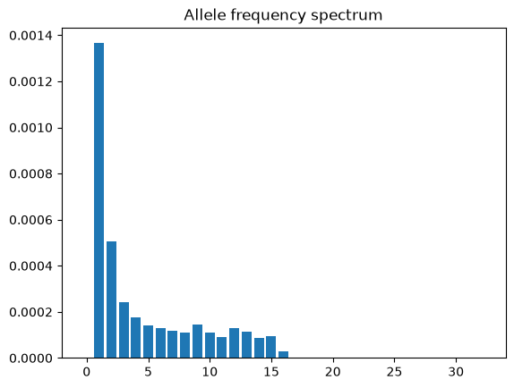
You can easily obtain the
TreeSequence.allele_frequency_spectrum() for the entire region (or for
windowed regions)
directly from the tree sequence (i.e. without needing to reconstruct genotypes)
afs = ts.allele_frequency_spectrum()
plt.bar(range(ts.num_samples + 1), afs)
plt.title("Allele frequency spectrum")
plt.show()
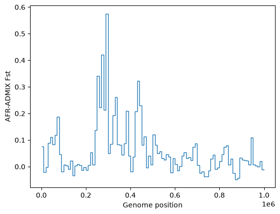
Similarly tskit allows fast and easy calculation of statistics along the genome. Here is a plot of windowed \(F_{st}\) between Africans and admixed Americans over this region of chromosome:
# Define the samples between which Fst will be calculated
pop_id = {p.metadata["name"]: p.id for p in ts.populations()}
sample_sets=[ts.samples(pop_id["AFR"]), ts.samples(pop_id["ADMIX"])]

# Do the windowed calculation, using windows of 10 kilobases
windows = list(range(0, int(ts.sequence_length + 1), 10_000))
F_st = ts.Fst(sample_sets, windows=windows)

# Plot
plt.stairs(F_st, windows, baseline=None)
plt.ylabel("AFR-ADMIX Fst")
plt.xlabel("Genome position")
plt.show()
Extracting the genetic tree at a specific genomic location is easy using tskit, which also provides methods to plot these trees. Here we grab the tree at position 10kb, and colour the different populations by grab the tree at position 10kb, and colour the samples according to their population, as described in the viz tutorial:
tree = ts.at(10_000)

colours = dict(AFR="yellow", EUR="cyan", ASIA="green", ADMIX="red")
styles = [
    f".leaf.p{pop.id} > .sym {{fill: {colours[pop.metadata['name']]}}}"
    for pop in ts.populations()
]

styles += [ # rotate the population labels, etc
    ".leaf > .lab {text-anchor: start; transform: rotate(90deg) translate(6px)}",
    ".leaf > .sym {stroke: black}"
]

labels = { # Label samples by population
    u: ts.population(ts.node(u).population).metadata["name"].capitalize()
    for u in ts.samples()
}

tree.draw_svg(
    size=(800, 500),
    canvas_size=(800, 520),
    node_labels=labels,
    style="".join(styles),
    y_axis=True,
    y_ticks=range(0, 30_000, 10_000)
)

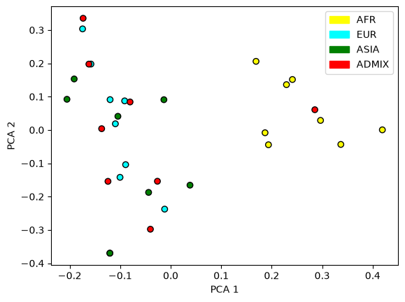
Or we can plot a principal components analysis of the genome, which should reflect geographical distinctiveness:
from matplotlib.patches import Patch

# Run the Principal Components Analysis (PCA)
pca_obj = ts.pca(num_components=2)

# Plot the PCA "factors"
col_list = [colours[pop.metadata["name"]] for pop in ts.populations()]
sample_pop_ids = ts.nodes_population[ts.samples()]
plt.scatter(*pca_obj.factors.T, c=[col_list[p] for p in sample_pop_ids], edgecolors= "black")
plt.xlabel("PCA 1")
plt.ylabel("PCA 2")
plt.legend(handles=[
    Patch(color=col_list[pop.id], label=pop.metadata["name"]) for pop in ts.populations()
]);
Population genetic inference#
If, instead of simulations, you want to analyse existing genomic data (for example stored in a VCF file), you will need to infer a tree sequence from it, using ARG inference software (such as SINGER, Relate, Threads, or tsinfer). Here we load an illustrative portion of a tree sequence inferred by tsinfer+tsdate which is based on about 7500 public human genomes, including genomes from the Thousand Genomes Project and Human Genome Diversity Project. The genomic region encoded in this tree sequence has been cut down to span positions 108Mb-110Mb of human chromosome 2, which spans the EDAR gene.
Note that we are using tszip.load() to load the file, as this
utility can also read and write compressed tree sequences in .tsz format.
import tszip
ts = tszip.load("data/unified_genealogy_2q_108Mb-110Mb.tsz")

# The ts encompasses a region on chr 2 with an interesting SNP (rs3827760) in the EDAR gene
edar_gene_bounds = [108_894_471, 108_989_220]  # In Mb from the start of chromosome 2
focal_variant = [v for v in ts.variants() if v.site.metadata.get("ID") == "rs3827760"].pop()
print("An interesting SNP within the EDAR gene:")
focal_variant
An interesting SNP within the EDAR gene:
|
|
|
|---|---|
| Site Id | 9 378 |
| Site Position | 1.0889714e+08 |
| Number of Nodes | 836 |
| Number of Alleles | 2 |
| Nodes with Allele 'A' | 384 (46%) |
| Nodes with Allele 'G' | 452 (54%) |
| Has Missing Data | False |
| Isolated as Missing | True |
For simplicity, this tree sequence has been simplified to include only those samples from the African and East Asian regions. These belong to a number of populations. The population information, as well as information describing the variable sites, is stored in tree sequence metadata:
import pandas as pd

print(ts.num_populations, "populations defined in the tree sequence:")

pop_names_regions = [
    [p.metadata.get("name"), p.metadata.get("region"), len(ts.samples(population=p.id))]
    for p in ts.populations()
]
with pd.option_context('display.max_rows', 100):
    display(pd.DataFrame(pop_names_regions, columns=["name", "region", "# genomes"]))
67 populations defined in the tree sequence:
| name | region | # genomes | |
|---|---|---|---|
| 0 | BantuKenya | AFRICA | 22 |
| 1 | BantuSouthAfrica | AFRICA | 16 |
| 2 | Biaka | AFRICA | 44 |
| 3 | Cambodian | EAST_ASIA | 18 |
| 4 | Dai | EAST_ASIA | 18 |
| 5 | Daur | EAST_ASIA | 18 |
| 6 | Han | EAST_ASIA | 66 |
| 7 | Hezhen | EAST_ASIA | 18 |
| 8 | Japanese | EAST_ASIA | 54 |
| 9 | Lahu | EAST_ASIA | 16 |
| 10 | Mandenka | AFRICA | 44 |
| 11 | Mbuti | AFRICA | 26 |
| 12 | Miao | EAST_ASIA | 20 |
| 13 | Mongolian | EAST_ASIA | 18 |
| 14 | Naxi | EAST_ASIA | 16 |
| 15 | NorthernHan | EAST_ASIA | 20 |
| 16 | Oroqen | EAST_ASIA | 18 |
| 17 | San | AFRICA | 12 |
| 18 | She | EAST_ASIA | 20 |
| 19 | Tu | EAST_ASIA | 20 |
| 20 | Tujia | EAST_ASIA | 18 |
| 21 | Xibo | EAST_ASIA | 18 |
| 22 | Yakut | EAST_ASIA | 50 |
| 23 | Yi | EAST_ASIA | 20 |
| 24 | Yoruba | AFRICA | 44 |
| 25 | Ami | EastAsia | 4 |
| 26 | Atayal | EastAsia | 2 |
| 27 | BantuHerero | Africa | 4 |
| 28 | BantuKenya | Africa | 4 |
| 29 | BantuTswana | Africa | 4 |
| 30 | Biaka | Africa | 4 |
| 31 | Burmese | EastAsia | 4 |
| 32 | Cambodian | EastAsia | 4 |
| 33 | Dai | EastAsia | 8 |
| 34 | Daur | EastAsia | 2 |
| 35 | Dinka | Africa | 6 |
| 36 | Esan | Africa | 4 |
| 37 | Gambian | Africa | 4 |
| 38 | Han | EastAsia | 6 |
| 39 | Hezhen | EastAsia | 4 |
| 40 | Japanese | EastAsia | 6 |
| 41 | Ju_hoan_North | Africa | 8 |
| 42 | Khomani_San | Africa | 4 |
| 43 | Kinh | EastAsia | 4 |
| 44 | Korean | EastAsia | 4 |
| 45 | Lahu | EastAsia | 4 |
| 46 | Luhya | Africa | 4 |
| 47 | Luo | Africa | 4 |
| 48 | Mandenka | Africa | 6 |
| 49 | Masai | Africa | 4 |
| 50 | Mbuti | Africa | 8 |
| 51 | Mende | Africa | 4 |
| 52 | Miao | EastAsia | 4 |
| 53 | Mozabite | Africa | 4 |
| 54 | Naxi | EastAsia | 4 |
| 55 | Oroqen | EastAsia | 4 |
| 56 | Saharawi | Africa | 4 |
| 57 | She | EastAsia | 4 |
| 58 | Somali | Africa | 2 |
| 59 | Thai | EastAsia | 4 |
| 60 | Tu | EastAsia | 4 |
| 61 | Tujia | EastAsia | 4 |
| 62 | Uygur | EastAsia | 4 |
| 63 | Xibo | EastAsia | 4 |
| 64 | Yi | EastAsia | 4 |
| 65 | Yoruba | Africa | 6 |
| 66 | Denisovan | None | 2 |
You can see that there are multiple African and East asian populations, grouped by region. Here we collect two lists of IDs for the sample nodes from the African region and from the East asian region:
sample_lists = {}
for n, rgns in {"Africa": {'AFRICA', 'Africa'}, "East asia": {'EAST_ASIA', 'EastAsia'}}.items():
    pop_ids = [p.id for p in ts.populations() if p.metadata.get("region") in rgns]
    sample_lists[n] = [u for p in pop_ids for u in ts.samples(population=p)]
With these lists we can calculate different windowed statistics
(here genetic diversity and
Tajima's D) within each of these regions:
edar_ts = ts.trim()  # remove regions with no data (changes the coordinate system)
windows = list(range(0, int(edar_ts.sequence_length)+1, 10_000))
data = {
    "Genetic diversity": {
        region: edar_ts.diversity(samples, windows=windows)
        for region, samples in sample_lists.items()
    },
    "Tajima's D": {
        region: edar_ts.Tajimas_D(samples, windows=windows)
        for region, samples in sample_lists.items()
    },
}

# Plot the `data`
fig, axes = plt.subplots(ncols=2, figsize=(15, 3))
start = ts.edges_left.min()  # the empty amount at the start of the tree sequence

for (title, plot_data), ax in zip(data.items(), axes):
    ax.set_title(title)
    ax.axvspan(edar_gene_bounds[0], edar_gene_bounds[1], color="lightgray")
    ax.axvline(focal_variant.site.position, ls=":")
    for label, stat in plot_data.items():
        ax.stairs(stat, windows+start, baseline=None, label=label)
    ax.text(edar_gene_bounds[0], 0, "EDAR")
    ax.legend()
plt.show()
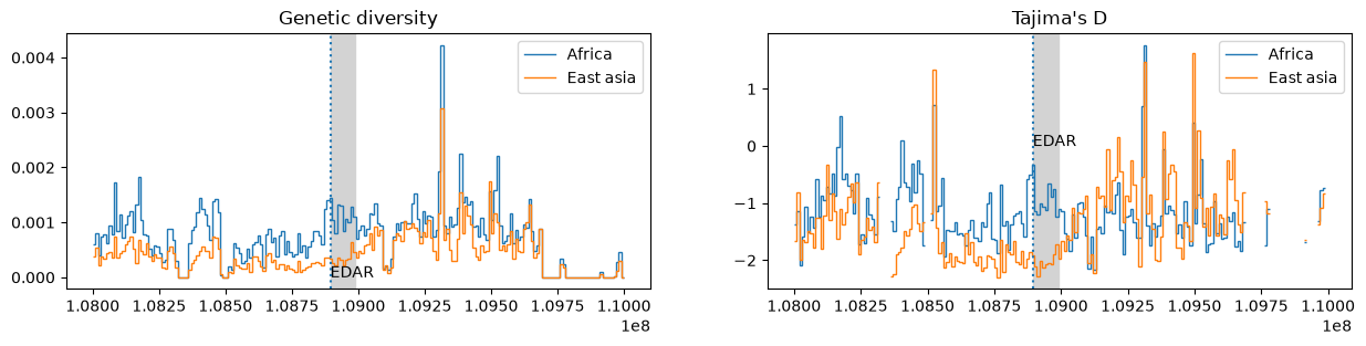
Other population genetic libraries such as scikit-allel (which is interoperable with tskit) could also have been used to produce the plot above. In this case, the advantage of using tree sequences is simply that they allow these sorts of analysis to scale to datasets of millions of whole genomes.
Topological analysis#
As this inferred tree sequence stores (an estimate of) the underlying genealogy, we can also derive statistics based on genealogical relationships. You may have noticed that this tree sequence also contains a sample genome based on an ancient genome, a Denisovan individual. We’ll first simplify the tree sequence to focus on only the Denisovan plus a common East Asian and a common African population:
# Focus on Han, San, and Denisovan
focal = {
    "Han": ts.samples(population=6),
    "San": ts.samples(population=17),
    "Denisovan": ts.samples(population=66),
}

for name, nodes in focal.items():  # Sanity check that we got the right IDs
    assert ts.population(ts.node(nodes[0]).population).metadata["name"] == name

# Simplify to just those samples ...
all_focal_samples = [u for samples in focal.values() for u in samples]
simplified_ts = ts.simplify(all_focal_samples, filter_sites=False)

# ... and find the tree around the rs3827760 SNP
focal_site = simplified_ts.site(focal_variant.site.id)
tree = simplified_ts.at(focal_site.position)
With this smaller number of samples, we can easily plot the tree at the “rs3827760” SNP:

You can see that the pair of magenta Denisovan genomes in this region tend to be more closely associated with the East Asian genomes. We can assess that by counting all the 3-tip topologies in the tree that contain one genome from each population:
topology_counter = tree.count_topologies()
embedded_topologies = topology_counter[range(simplified_ts.num_populations)]

See Counting topologies for an introduction to topological methods in tskit.
Further information#
This brief introduction is meant as a simple taster. Many other efficient population genetic analyses are possible when you have genomic data stored as a tree sequence.
The rest of the tutorials contain a large number of examples which are relevant to population genetic analysis and research. You can also visit the learning section of the tskit website.