Visualization#
Yan Wong
It is often helpful to visualize a single tree — or multiple trees along a tree sequence — together with sites and mutations. Tskit provides methods to do this, outputting either plain ascii or unicode text, or the more flexible Scalable Vector Graphics (SVG) format. The first two sections of this tutorial give details of these methods, using a few 50kb tree sequences generated by msprime as examples: one in which selection has occurred, and others which involve subdivision into 3 populations (labelled A, B, and C).
If you just want a quick look at visualization possibilities, you might want to skip the explanations and just browse some Examples, which contain fully reproducible code.
Note
This tutorial is primarily focussed on showing a tree sequence as a set of marginal trees along a genome. The section titled Other visualizations provides examples of other representations of tree sequences, or the processes that can create them.
Additionally, other software tools exist that can plot genealogies (ARGs) in tree sequence format. For example, in these tutorials we use the tskit_arg_visualizer tool to provide simple graph-centric visualizations. You might also want to explore tools such as ARGscape, Lorax, tsbrowse, or even high-level analysis tools like TwisstNTern.
Text format#
The TreeSequence.draw_text() and
Tree.draw_text() methods provide
a quick way to print out a tree sequence, or an individual tree within it. They are
primarily useful for looking at topologies in small datasets (e.g. fewer than 20 sampled
genomes), and do not display mutations.
# Print a tree sequence
print(ts_tiny.draw_text())

print("The first tree in the tree sequence above, but replacing some node ids with names:")
print(ts_tiny.first().draw_text(
    # An example of how to change or omit node labels: unspecified nodes are omitted
    # The same convention applies to SVG graphics
    node_labels={0: "Alice", 1: "Bob", 2:"Chris", 3: "Dora", 6: "MRCA"}
))
11428.48┊         ┊         ┊         ┊         ┊   13    ┊         ┊         ┊         ┊
        ┊         ┊         ┊         ┊         ┊  ┏━┻━┓  ┊         ┊         ┊         ┊
11144.74┊         ┊         ┊         ┊         ┊  ┃   ┃  ┊   12    ┊         ┊         ┊
        ┊         ┊         ┊         ┊         ┊  ┃   ┃  ┊  ┏━┻━┓  ┊         ┊         ┊
9753.69 ┊         ┊         ┊         ┊         ┊  ┃   ┃  ┊  ┃   ┃  ┊   11    ┊         ┊
        ┊         ┊         ┊         ┊         ┊  ┃   ┃  ┊  ┃   ┃  ┊  ┏━┻━┓  ┊         ┊
6204.42 ┊         ┊         ┊         ┊   10    ┊  ┃   ┃  ┊  ┃   ┃  ┊  ┃   ┃  ┊         ┊
        ┊         ┊         ┊         ┊  ┏━┻━┓  ┊  ┃   ┃  ┊  ┃   ┃  ┊  ┃   ┃  ┊         ┊
3893.05 ┊         ┊         ┊         ┊  ┃   ┃  ┊  ┃   ┃  ┊  ┃   ┃  ┊  ┃   ┃  ┊    9    ┊
        ┊         ┊         ┊         ┊  ┃   ┃  ┊  ┃   ┃  ┊  ┃   ┃  ┊  ┃   ┃  ┊  ┏━┻━┓  ┊
3378.92 ┊         ┊    8    ┊    8    ┊  ┃   ┃  ┊  ┃   ┃  ┊  ┃   ┃  ┊  ┃   ┃  ┊  ┃   ┃  ┊
        ┊         ┊  ┏━┻━┓  ┊  ┏━┻━┓  ┊  ┃   ┃  ┊  ┃   ┃  ┊  ┃   ┃  ┊  ┃   ┃  ┊  ┃   ┃  ┊
2076.43 ┊         ┊  ┃   ┃  ┊  7   ┃  ┊  7   ┃  ┊  7   ┃  ┊  7   ┃  ┊  7   ┃  ┊  7   ┃  ┊
        ┊         ┊  ┃   ┃  ┊ ┏┻┓  ┃  ┊ ┏┻┓  ┃  ┊ ┏┻┓  ┃  ┊ ┏┻┓  ┃  ┊ ┏┻┓  ┃  ┊ ┏┻┓  ┃  ┊
1941.72 ┊   6     ┊  6   ┃  ┊ ┃ ┃  ┃  ┊ ┃ ┃  ┃  ┊ ┃ ┃  ┃  ┊ ┃ ┃  ┃  ┊ ┃ ┃  ┃  ┊ ┃ ┃  ┃  ┊
        ┊ ┏━┻━┓   ┊ ┏┻┓  ┃  ┊ ┃ ┃  ┃  ┊ ┃ ┃  ┃  ┊ ┃ ┃  ┃  ┊ ┃ ┃  ┃  ┊ ┃ ┃  ┃  ┊ ┃ ┃  ┃  ┊
1439.14 ┊ ┃   5   ┊ ┃ ┃  ┃  ┊ ┃ ┃  ┃  ┊ ┃ ┃  ┃  ┊ ┃ ┃  ┃  ┊ ┃ ┃  ┃  ┊ ┃ ┃  ┃  ┊ ┃ ┃  ┃  ┊
        ┊ ┃ ┏━┻┓  ┊ ┃ ┃  ┃  ┊ ┃ ┃  ┃  ┊ ┃ ┃  ┃  ┊ ┃ ┃  ┃  ┊ ┃ ┃  ┃  ┊ ┃ ┃  ┃  ┊ ┃ ┃  ┃  ┊
33.99   ┊ ┃ ┃  4  ┊ ┃ ┃  4  ┊ ┃ ┃  4  ┊ ┃ ┃  4  ┊ ┃ ┃  4  ┊ ┃ ┃  4  ┊ ┃ ┃  4  ┊ ┃ ┃  4  ┊
        ┊ ┃ ┃ ┏┻┓ ┊ ┃ ┃ ┏┻┓ ┊ ┃ ┃ ┏┻┓ ┊ ┃ ┃ ┏┻┓ ┊ ┃ ┃ ┏┻┓ ┊ ┃ ┃ ┏┻┓ ┊ ┃ ┃ ┏┻┓ ┊ ┃ ┃ ┏┻┓ ┊
0.00    ┊ 0 1 2 3 ┊ 0 1 2 3 ┊ 0 1 2 3 ┊ 0 1 2 3 ┊ 0 1 2 3 ┊ 0 1 2 3 ┊ 0 1 2 3 ┊ 0 1 2 3 ┊
        0       9855      13901     21285     23424     25213     30463     46237     50000

The first tree in the tree sequence above, but replacing some node ids with names:
    MRCA
  ┏━━━┻━━━━┓
  ┃        ┃
  ┃    ┏━━━┻━━━┓
  ┃    ┃       ┃
  ┃    ┃    ┏━━┻━━┓
Alice Bob Chris Dora
SVG format#
Most users will want to use the SVG drawing functions
TreeSequence.draw_svg() and
Tree.draw_svg() for visualization. Being a vectorised
format, SVG files are suitable for presentations, publication, and
editing or converting to other graphic formats; some
basic forms of animation are also possible. Both functions produce an SVG string which is
automatically drawn if the string is the result of the last call in a Jupyter notebook:
from IPython.display import display
svg_size = (800, 250) # Height and width for the SVG: optional but useful for this notebook
svg_string = ts_tiny.draw_svg(
    size=svg_size,
    y_axis=True, y_label=" ",  # optional: show a time scale on the left
    time_scale="rank", x_scale="treewise",  # Force same axis settings as the text view
    title="A basic SVG plot",
)
display(svg_string)  # If the last line in a cell, wrapping this in display() is not needed

By default, sample nodes are drawn as black squares, and non-sample nodes are drawn as black circles (but see below for ways to e.g. hide or colour these node symbols - NB. apologies to US readers: the British spelling of “colour” will be used in the rest of this tutorial).
Axes and scales#
For ease of drawing, the text representation and the SVG image above use unconventional non-linear X and Y coordinate systems. By default, the SVG output uses a more conventional linear scale for both time (Y) and genome position (X), and indicates the position of each tree along the genome by an alternating shaded background. Although more intuitive, linear scales can obscure some features of the trees, for example causing labels to overlap:
ts_tiny.draw_svg(size=svg_size, y_axis=True)

One way to avoid overlapping labels on the Y axis is to use the y_ticks parameter,
which will be used in most subsequent examples in this tutorial.
Larger tree sequences#
So far, we have plotted only very small tree sequences. To visualize larger tree
sequences it is sometimes advisable to focus on a small region of the genome, possibly
even a single tree. The x_lim parameter allows you to plot the part of a tree
sequence that spans a particular genomic region: here’s a slightly larger tree sequence
with 8 samples, but where we’ve restricted the amount of the tree sequence we plot:
x_limits = [5000, 15000]
# Create evenly-spaced y tick positions to avoid overlap
y_tick_pos = [0, 1000, 2000, 3000]

display(ts_small.draw_svg(
    size=svg_size,
    y_axis=True,
    y_ticks=y_tick_pos,
    x_lim=x_limits,
    title="The tree sequence between positions {} and {}".format(*x_limits)
))

third_tree = ts_small.at_index(2)
display(third_tree.draw_svg(title="A plot of the third tree"))


As the number of sample nodes increases, internal nodes often bunch up at recent time
points, obscuring relationships. Setting time_scale="rank", as in the first SVG plot,
is one way to solve this. Another is to use a log-scale on the time axis, which can be
done by specifying time_scale="log_time", as below. To compare node times across the
plot, this example also uses the y_gridlines option, which puts a very faint grid
line at each y tick (if you are finding the lines difficult to see, note that the line
intensity, along with many other plot features, can be modified through
styling, which we also use in this example to avoid
overlapping text by shrinking the node labels and rotating those associated with leaves;
styling is detailed later in this tutorial).
wide_fmt = (1200, 280)
# Create a stylesheet that shrinks labels and rotates leaf labels, to avoid overlap
node_label_style = (
    ".node > .lab {font-size: 80%}"
    ".leaf > .lab {text-anchor: start; transform: rotate(90deg) translate(6px)}"
)

ts_full.first().draw_svg(
    size=wide_fmt,
    time_scale="log_time",
    y_gridlines=True,
    y_axis=True,
    y_ticks=[1, 10, 100, 1000],
    style=node_label_style + "svg > .title text {font-size: 150%}",
    title="A larger tree, on a log timescale",
)

For even larger numbers of samples, you can plot the trees for a subset of samples
by applying the TreeSequence.simplify() method (make sure to specify
filter_nodes=False to retain the same node IDs). For a fancier solution, see
Simplifying larger plots below.
Plotting mutations#
By default the SVG visualization also plots sites and mutations on the tree or
tree sequence (this can be disabled using the omit_sites parameter). For example,
adding mutations to the 8-sample tree sequence above gives the following plot: each
mutation is marked by a red cross on the branch where it occurs. Symbols are
either placed at the mutation’s known time, or (if the mutation time is unknown or
the time_scale parameter has been set to "rank") spaced evenly along the branch.
By default, each mutation is also labelled with its mutation ID.
If the X axis is shown (which it is by default when drawing a tree sequence, but not when drawing an individual tree) then the sites are plotted using a black tickmark above the axis line. Each plotted mutation at the site is then overlaid on top of this as a red downwards-pointing chevron.
ts_mutated = msprime.sim_mutations(ts_small, rate=1e-7, random_seed=342)
ts_mutated.draw_svg(y_axis=True, y_ticks=y_tick_pos, x_lim=x_limits)

Note that, unusually, the rightmost site on the axis has more than one stacked chevron, indicating that multiple mutations in the tree occur at the same site. These could be mutations to different allelic states, or recurrent/back mutations. In this case the mutations, 14 and 15 (above nodes 1 and 6) are recurrent mutations from T to G.
Site(id=14, position=13963.0, ancestral_state='T', mutations=[
  Mutation(id=14, site=14, node=1, derived_state='G', parent=-1, metadata=b'', time=619.6499091610359, edge=14, inherited_state='T'),
  Mutation(id=15, site=14, node=6, derived_state='G', parent=-1, metadata=b'', time=370.24979591084764, edge=4, inherited_state='T')],
 metadata=b'')
Which mutations are shown?#
When using the x_lim parameter, only the mutations in the plotted region are shown.
For the third tree in the tree sequence visualization above, we thus haven’t plotted
mutations above position 15000. We can see all the mutations in the tree by changing the
plot region, or simply plotting the tree itself:
tree3 = ts_mutated.at_index(2)
tree3.draw_svg(
    size=(300, 300),
    title=f"Third tree, from {int(tree3.interval.left)} bp to {int(tree3.interval.right)} bp",
)

However, when plotting a single tree it may not be evident that identical branches
may exist in several adjacent trees, indicating an edge
that persists across adjacent trees. For instance the rightmost branch in the tree above,
from node 10 down to 7, exists in the previous two trees too. Indeed, this edge has a
mutation on it at position 6295, in the first tree. This mutation is not plotted in the
tree above, but if you want all the mutations on each edge to be plotted, you can set
the all_edge_mutations parameter to True. This adds any extra mutations that are
associated with an edge in the tree but which fall outside the interval of that tree; by
default these mutations are drawn in a slightly different shade (e.g. mutation 64 below).
tree3.draw_svg(
    size=(300, 300),
    all_edge_mutations=True,
    title=(
        '<tspan dy="12">Third tree as above, but with</tspan>'
        '<tspan dy="13" x="0">visible edges showing all mutations</tspan>'
    )
)

Labelling and annotation#
Although the default node and mutation labels show unique identifiers, they aren’t
terribly intuituive. The node_labels and mutation_labels parameters can be used
to set more meaningful labels (for example from the tree sequence Metadata).
See Dynamic effects if you want to dynamically hide and show such
labels.
nd_labels = {  # An array of labels for the nodes
    # Set sample node labels from metadata. Here we use the population name, but you might want
    # to use the *individual* name instead, if the individuals in your tree sequence have names
    n.id: ts_mutated.population(n.population).metadata["name"]
    for n in ts_mutated.nodes()
    if n.is_sample()
}

mut_labels = { # An array of labels for the mutations
    mut.id: f"{mut.inherited_state}→{mut.derived_state}" for mut in ts_mutated.mutations()
}

ts_mutated.draw_svg(
    size=(1000, 300),
    y_axis=True, y_ticks=y_tick_pos, x_lim=x_limits,
    node_labels=nd_labels,
    mutation_labels=mut_labels,
)

Annotating genome regions#
To annotate genomic regions along the X axis of the tree sequence plot, you can pass a
dictionary of x_regions, mapping (start, end) tuples to labels. Below we have also
used css to hide all but the first and last x axis tick label to avoid visual clashing,
and hidden all the mutation and node labels by setting them to {}:
x_regions = {(5_000, 12_000): "Gene 1", (21_123, 33_321): "Gene 2"}
hide_internal_x_tick_labels = (
    ".x-axis .tick .lab {visibility: hidden}"
    ".x-axis .tick:first-of-type .lab, .x-axis .tick:last-of-type .lab  {visibility: visible}"
    ".x-regions .r1 rect {fill: cyan}"  # 2nd region (ID 1) tagged with class="r1"
)
ts_mutated.draw_svg(
    size=(1000, 300),
    y_axis=True,
    y_ticks=range(0, int(ts_mutated.max_time), 1000),
    node_labels={},
    mutation_labels={},
    style=hide_internal_x_tick_labels,
    x_regions=x_regions,
)

Arbitrary annotation#
It is also possible to add arbitrary annotations to the SVG plot, as detailed in the next section. To locate positions for annotation, see the examples in SVG plot internals.
Adding bespoke SVG#
The preamble option allows arbitrary SVG text to be added at the start of the plot.
This can be useful to annotate plots, produce legends, etc. although it requires some
knowledge of the SVG graphics language (see the Legend example
later in this tutorial for a node colour legend).
mut_labels = {
mut.id: f"{mut.inherited_state}{int(site.position)}{mut.derived_state}"
for site in ts_mutated.sites() for mut in site.mutations
}
svg_text=(
'<rect x="30" y="267" height="30" width="245" fill="lightgrey" stroke="black" />'
'<text font-size="12" text-anchor="middle" y="280" fill="red">'
'<tspan font-size="14" x="150" fill="darkred" font-weight="bold">Mutation labels:</tspan>'
'<tspan dy="1em" x="150"><inherited_state><POSITION><derived_state></tspan>'
'</text>'
)
ts_mutated.draw_svg(
size=(800, 300),
title="A plot with a rudimentary legend to describe the mutation label format",
y_axis=True, y_ticks=y_tick_pos, x_lim=x_limits,
node_labels=nd_labels,
mutation_labels=mut_labels,
preamble=svg_text,
)

Plotting side-by-side#
As any conceivable SVG commands can be added (including nesting one SVG inside another),
using preamble is extremely flexible, but can be fiddly. You can, for example, plot
one tree next to a completely different one by adding one into the preamble of the other.
This is demonstrated in the helper function below. It adds space into the first
plot without rescaling the image itself by using the canvas_size parameter. Further
plots are then added into the preamble, moved to the left using
root_svg_attributes={"x", x_offset}.
def draw_svg_side_by_side(
    drawables,
    *,
    size=(200, 200),
    sizes=None,
    padding=40,
    canvas_size=None,
    per_svg_kwargs=None,
    **kwargs,
):
    """
    Plot multiple Tree or TreeSequence objects side-by-side by embedding the SVG for
    each later object in the preamble of the first.

    :param list drawables: A list of Tree or TreeSequence objects.
    :param tuple size: The size of each individual SVG plot, if `sizes` is not given.
    :param list sizes: An optional list of sizes, one per plot.
    :param int padding: The horizontal gap between adjacent plots.
    :param tuple canvas_size: The overall canvas size. If None, infer it from `size`.
    :param list per_svg_kwargs: An optional list of dicts of keyword arguments to pass
        to each individual `draw_svg` call. These are merged on top of `**kwargs`.
    :param kwargs: Common keyword arguments passed to each `draw_svg` call.
    """
    if len(drawables) == 0:
        raise ValueError("Need at least one drawable")
    if per_svg_kwargs is None:
        per_svg_kwargs = [{} for _ in drawables]
    if len(per_svg_kwargs) != len(drawables):
        raise ValueError("per_svg_kwargs must have the same length as drawables")
    if sizes is None:
        sizes = [size for _ in drawables]
    if len(sizes) != len(drawables):
        raise ValueError("sizes must have the same length as drawables")
    if canvas_size is None:
        canvas_size = (
            sum(s[0] for s in sizes) + (len(drawables) - 1) * padding,
            max(s[1] for s in sizes),
        )

    preamble = []
    x_offset = sizes[0][0] + padding
    for j, drawable in enumerate(drawables[1:], start=1):
        svg_kwargs = dict(kwargs)
        svg_kwargs.update(per_svg_kwargs[j])
        svg_kwargs["size"] = sizes[j]
        svg_kwargs["root_svg_attributes"] = {
            **svg_kwargs.get("root_svg_attributes", {}),
            "x": x_offset,
        }
        preamble.append(drawable.draw_svg(**svg_kwargs))
        x_offset += sizes[j][0] + padding

    first_kwargs = dict(kwargs)
    first_kwargs.update(per_svg_kwargs[0])
    first_kwargs["size"] = sizes[0]
    first_kwargs["canvas_size"] = canvas_size
    first_kwargs["preamble"] = first_kwargs.get("preamble", "") + "".join(preamble)
    return drawables[0].draw_svg(**first_kwargs)
draw_svg_side_by_side(
    [tree3, tree3],  # these could be different trees from different tree sequences
    size=(300, 300),
    per_svg_kwargs=[{"title": "3rd tree"}, {"title": "3rd tree, no sites", "omit_sites": True}],
)

Visually reordering nodes#
As tskit is not primarily a visualization library, there are no methods for rotating branches when visualizing specific trees. Moreover, a tidy arrangement for one tree could be a poor arrangement for an adjacent tree in the tree sequence.
However, because the default ordering is to put lower numbered leaves to the left,
it is possible to obtain an arbitrary ordering by changing the node IDs
as required (e.g. using the subset method). If you are labelling nodes using
metadata, this will all be fine, but if you are using the default ID labelling scheme,
you’ll should provide labels that map back to the original IDs, to avoid confusion.
Here’s an example, using a generic reordering function to reverse the visual order of nodes 0…4 ()
import numpy as np

def reorder_leaves(tree, leaf_order_ids):
    # Return a new tree in an identical tree sequence but with the node IDs
    # swapped to draw leaf order as close possible to the provided leaf_order_ids
    # You will need to plot the node labels using metadata or the returned node_map
    ts = tree.tree_sequence
    all_nodes = np.arange(ts.num_nodes)
    leaves = [u for u in tree.nodes(order="minlex_postorder") if tree.is_leaf(u)]
    all_nodes[leaves] = leaf_order_ids
    reorder_ts = ts.subset(all_nodes, reorder_populations=False, remove_unreferenced=False)
    return reorder_ts.at_index(tree.index), all_nodes

# swap the order of 0, 1, 2, 3, 4
orig_tree = ts_mutated.first()
new_tree, node_map = reorder_leaves(orig_tree, [4, 3, 2, 1, 0, 5, 7, 6])

draw_svg_side_by_side(
    [orig_tree, new_tree],
    per_svg_kwargs=[
        {"title": "Original tree"},
        {"title": "Leaf nodes reordered", "node_labels": {u: v for u, v in enumerate(node_map)}},
    ],
)

This approach can be used to define functions to plot ladderized trees, see e.g. this GitHub discussion.
Styling#
The SVG output produced by tskit contains a large number of
classes which can be used to
target different elements of the drawing, allowing them to be hidden, styled, or
otherwise manipulated. This is done by passing a
cascading style sheet (CSS) string to
draw_svg. A common use of styles is to colour nodes by their population:
styles = []
# Create a style for each population, programmatically (or just type the string by hand)
for colour, p in zip(['red', 'green', 'blue'], ts_full.populations()):
    # target the symbols only (class "sym")
    s = f".node.p{p.id} > .sym " + "{" + f"fill: {colour}" + "}"
    styles.append(s)
    print(f'"{s}" applies to nodes from population {p.metadata["name"]} (id {p.id})')
css_string = " ".join(styles)
print(f'CSS string applied:\n    "{css_string}"')

ts_full.first().draw_svg(
    size=wide_fmt,
    node_labels={},    # Remove all node labels for a clearer viz
    style=css_string,  # Apply the stylesheet
)
".node.p0 > .sym {fill: red}" applies to nodes from population A (id 0)
".node.p1 > .sym {fill: green}" applies to nodes from population B (id 1)
".node.p2 > .sym {fill: blue}" applies to nodes from population C (id 2)
CSS string applied:
    ".node.p0 > .sym {fill: red} .node.p1 > .sym {fill: green} .node.p2 > .sym {fill: blue}"

Colouring nodes by population makes it immediately clear that, while the tree structure does not exactly reflect the population divisions, there’s still considerable population substructure present in this larger tree.
Todo
The (older) Tree.draw() function also has a node_colour argument that can be
used to colour tree nodes, which is used in some of the other tskit tutorials. Under the
hood, this function simply sets appropriate SVG styles on nodes. We intend to make it
easier to set colours in a similar way: see https://github.com/tskit-dev/tskit/issues/579.
The CSS string used to style the tree above takes advantage of the general classes defined
in a tskit SVG file: a node symbol always has a class named sym, which is contained
within a grouping element of class
node. Moreover, elements such as node have additional classes, such as p1,
indicating that the node in this case belongs to the population with ID 1.
Available css classes#
Here are the css classes in a tskit SVG which can be used to style specific elements.
Within the plotting area#
tree: a grouping element containing each treenode: a grouping element within a tree, containing a node and its descendant elements such as a node symbol, an edge, mutations, and other nodes.mut: a grouping element containing a mutation symbol and labelextra: an extra class for mutations outside the treelab: a label element (for a node, mutation, axis, tick number, etc.)sym: a symbol element (e.g. a node, mutation, or site symbol)edge: an edge element (i.e. a branch in a tree)root,leafandsample: additional classes applied to a node group if the node is a root node, a leaf node or a sample nodeunknown_time: a class added tomutgroups if the time of the mutation istskit.UNKNOWN_TIME.rgtandlft: additional classes applied to labels for left- or right-justification
Outside the plotting area#
axes: a grouping element containing the X and Y axes, if either are presentx-axis,y-axis: more specific grouping elements contained withinaxestick: a single tick on an axis, containing a tickmark line and a labelsite: a grouping element representing a site (plotted on the X axis), containing a site symbol (a tick line) and zero or moremutgroups, each containing a chevron-shaped mutation symbolbackground: the shaded background of a tree sequence plotgrid: a gridline
ID-based classes#
Elements have additional classes based on the IDs of trees, edges, nodes,
parent (ancestor) nodes, individuals, populations, mutations, and sites.
These class names start with a single letter (respectively
t, e, n, a, i, p, m, and s) followed by a
numerical ID. For example, here’s a typical node in a tskit SVG plot:
<g class="a10 i3 leaf m16 m17 node n7 p2 s15 s16 sample">...</g>
This corresponds to node 7, the rightmost leaf in the third tree in the mutated tree
sequence (plotted in the previous section but one). The classes indicate that it
has an immediate ancestor (parent) node with ID 10 (a10), and that the node
belongs to an individual with ID 3 (i3).
The classes n7 and p2 tell us that the node ID is 7 and is from the
population with ID 2 (p2). Other ID classes on the node tell us about the mutations
above that node, of which there are two in this case, with
IDs 16 and 17 (m16, m17); those mutations are associated with
site IDs 15 and 16 (s16, s17).
Other grouping elements apart from nodes can also contain ID-based classes. For example
the tree group contains the ID of the tree (e.g. t0), the site group on the X axis
contains the site ID (e.g. s15) the mut class contains the mutation ID (e.g. m16),
and so on.
CSS selector quick reference#
If you don’t do this all the time it’s not easy to remember what the various separators mean, so here’s a quick reference (for more, see these docs):
abc(Typeabc, likegfor a<g>...</g>tag).xyz(Classxyz)#uvw(IDuvw),(Selector list, means “or”)>(Child combinator)“
+(Next-sibling combinator)~(Subsequent sibling combinator)|(Namespace separator)
Styling graphical elements#
The classes above make it easy to target specific nodes or edges in one or multiple trees. For example, we can colour branches that are shared between trees:
css_string = ".a15.n9 > .edge {stroke: cyan; stroke-width: 2px}"  # branches from 15->9
ts_small.draw_svg(time_scale="rank", size=wide_fmt, style=css_string)

Or rather than identifying shared branches using the same parent and child, you can use the edge ID, which allows effects like colouring the edges by their span, to emphasize the routes through which more genomic information has been inherited. Below we do this for a single tree, which avoids making a styling rule for every edge in the tree sequence:
tree = ts_small.at_index(2)
edges = tree.edge_array[tree.edge_array != tskit.NULL]
spans = tree.tree_sequence.edges_right[edges] - tree.tree_sequence.edges_left[edges]
values = ((1-spans/spans.max()) * 255).astype(int)
style = "".join([f".edge.e{e} {{stroke:#{v:02X}{v:02X}{v:02X}}}" for e, v in zip(edges, values)])
tree.draw_svg(style=style + ".edge {stroke-width: 2px}")

By generating the css string programatically, you can target all the edges present in a particular tree, and see how they gradually disappear from adjacent trees. Below, for example the branches in the central tree have been coloured red, as have the identical branches in adjacent trees. The central tree represents a location in the genome that has seen a selective sweep, and therefore has short branch lengths: adjacent trees are not under direct selection and thus the black branches tend to be longer. These (red) shared branches extending far on either side represent shared haplotypes, and this shows how long, shared haplotypes can extend much further away from a sweep than the region of reduced diversity (which is the region spanned by the short tree in the middle). For visual clarity, node symbols and labels have been turned off.
css_edge_targets = []  # collect the css targets of all the edges in the selected tree
sweep_location = ts_selection.sequence_length / 2  # NB: sweep is in the middle of the ts
focal_tree = ts_selection.at(sweep_location)
for node_id in focal_tree.nodes():
    parent_id = focal_tree.parent(node_id)
    if parent_id != tskit.NULL:
        css_edge_targets.append(f".a{parent_id}.n{node_id}>.edge")
css_string = ",".join(css_edge_targets) + "{stroke: red} .sym {display: none}"
css_string += (  # Rotate the position labels etc
    ".x-axis .ticks .lab {text-anchor: start; transform: translate(6px) rotate(90deg)}"
    ".x-axis .title .lab {text-anchor: start}"
)
wide_tall_fmt = (1200, 400)
ts_selection.draw_svg(
    style=css_string,
    size=wide_tall_fmt,
    canvas_size=(wide_tall_fmt[0], wide_tall_fmt[1] + 30),
    x_lim=[1e4, 4e4],
    node_labels={},
)

Note
Branches in multiple trees that have the same parent and child do not always correspond to a single edge in a tree sequence: for example, edges have the additional constraint that they must belong to adjacent trees.
Dynamic effects#
In the previous example, the large size of the plotted trees meant that, for clarity,
the node and mutation labels were turned off (in that case by passing empty mappings
to the node_labels and mutation_labels parameters). Nevertheless, it can be useful
to identify nodes and mutations, and this can be done dynamically (on “mouseover”) by
setting the CSS display
property to none vs initial, and combining it with the CSS :hover pseudoclass.
Here’s an example using a region from within the previous example:
from IPython.display import HTML
# add some mutations
ts = msprime.sim_mutations(ts_selection, rate=2e-8, random_seed=1)

node_label_css = (
    # hide node labels by default
    "#hover_example .node > .sym ~ .lab {display: none}"
    # Unless the adjacent node or the label is hovered over
    "#hover_example .node > .sym:hover ~ .lab {display: inherit}"
    "#hover_example .node > .sym ~ .lab:hover {display: inherit}"
)

mut_label_css = (
    # hide mutation labels by default
    "#hover_example .mut .sym ~ .lab {display: none}"
    # Unless the adjacent node or the label is hovered over
    "#hover_example .mut .sym:hover ~ .lab {display: inherit}"
    "#hover_example .mut .sym ~ .lab:hover {display: inherit}"
)

optional_css = (
    # These are optional, but setting e.g. the node label text to bold with grey stroke
    # and a black fill, serves to make black text readable against a black tree
    "svg#hover_example {background-color: white}"
    "#hover_example .tree .plotbox .lab {stroke: #CCC; fill: black; font-weight: bold}"
    "#hover_example .tree .mut .lab {stroke: #FCC; fill: red; font-weight: bold}"
)

HTML(ts.draw_svg(
    style=optional_css + node_label_css + mut_label_css,
    y_axis=True,
    y_ticks={0: "0", 500: "", 1000: "1000"},
    x_lim=[2.3e4, 2.7e4],
    root_svg_attributes={"id": "hover_example"},
        # Label node by name in metadata, if it exists, else node ID
    node_labels={u.id: u.metadata.get("name", f"NodeID={u.id}") for u in ts.nodes()},
    mutation_labels={
        # Label mutation by site position, prev state, and new state
        m.id: (
            f"pos {s.position:g}: " +
            (s.ancestral_state if m.parent<0 else ts.mutation(m.parent).derived_state) +
            f"→{m.derived_state}"
        )
        for s in ts.sites()
        for m in s.mutations
    },
))
Note
Above we have wrapped the svg in an IPython HTML
class, and given the SVG a unique
id as described below in More about styling. This forces the SVG
plot to be rendered inline (rather than inside an <img> tag), allowing the hover
functionality to work in all supported Jupyter notebook implementations. However,
depending on your Jupyter setup, the HTML() wrapper may not be necessary.
Using the transformations discussed in the next section, it is also possible to animate SVG images, as shown in the Animation code within the SVG examples section near the end of this tutorial.
Transforming and masking elements#
We can also use styles to transform elements of the drawing, shifting them into different locations or changing their orientation. For example, earlier in this tutorial we used the following CSS string to rotate leaf labels:
.leaf > .lab {text-anchor: start; transform: rotate(90deg) translate(6px)}
Transformations not only allow us to shift elements about, but also resize and skew them. When applied to both symbols and labels this can create rather different formatting styles:
css_string = (
    # Draw large yellow circles for nodes ...
    ".node > .sym {transform: scale(2.2); fill: yellow; stroke: black; stroke-width: 0.5px}"

    # ...but for leaf nodes, override the yellow circle using a more specific CSS target
    ".node.leaf > .sym {transform: scale(1); fill:black}"

    # Override default node text position to be based at (0, 0) relative to the node pos
    # Note that the .tree specifier is needed to make this more specific than the default
    # positioning which is targeted at ".lab.lft" and ".lab.rgt"
    ".tree .node > .lab {transform: translate(0, 0); text-anchor: middle; font-size: 7pt}"

    # For leaf nodes, override the above positioning using a subsequent CSS style
    ".node.leaf > .lab {transform: translate(0, 12px); font-size: 10pt}"
)
ts_small.first().draw_svg(style=css_string)

Note that when transforming elements, parts of the drawing may be plotted outsize of
of the standard canvas, so the canvas_size option is particularly useful
when performing more radical CSS transformations, for example to create
3D effects:
skew = 0.8  # How skewed the trees are, in radians

# CSS transforms used to skew the trees
style = f".tree .plotbox {{transform: skewY({skew}rad)}}"
# Shift the x axis to make room for the skewed trees
shift_axis = (10, 50)
style += f".x-axis {{transform: translate({shift_axis[0]}px, {shift_axis[1]}px)}}"

# Must define a bigger canvas size so we don't crop the axis off
size = (800, 200) # width, height of svg
canvas_size = (size[0] + shift_axis[0], size[1] + shift_axis[1])

ts_tiny.draw_svg(size=size, x_scale="treewise", style=style, canvas_size=canvas_size)

Note
Using transform in styles is an SVG2 feature, and has not yet been implemented in
the software programs Inkscape or librsvg. Therefore if you are
converting or editing the examples above, the
transformed elements may be positioned incorrectly. For changing symbols, the
symbol_size option can be used to simply change the size of all symbols in the plot,
but otherwise you may need to use the chromium workaround documented
here.
Although it is hard to change the style of a node symbol, the visible area of the symbol
can be modified using the clip-path CSS property. This can be useful to show, for
instance, a triangle to summarise the descendants of a MRCA.
# Check that MRCA of 2 & 3 is node 4 in all trees, assumed later
assert all([4 == tree.mrca(2, 3) for tree in ts_tiny.trees()])

styles = [
    # Set all node labels to be rotated and small
    ".node > .lab {text-anchor: start; transform: rotate(90deg) translate(6px); font-size: 8px}",

    # Hide all nodes descending from node 4. We then treat node 4 as a summary node
    ".n4 > .node {display: none}",

    # Use clipping & scaling to change the symbol for node 4 into a summary triangle
    ".n4 > .sym {clip-path: polygon(50% 50%, 75% 75%, 25% 75%); transform: scale(8.0, 8.0)}",

    # Make the font bigger for this summary node label
    ".n4 > .lab {transform: rotate(90deg) translate(14px); font-size: 16px}"
]

node_labels = {0: "Nd. 0", 1: "Nd. 1", 4: "Two samples"}

ts_tiny.draw_svg(
    size=(800, 300),
    x_scale="treewise",
    time_scale="log_time",
    style="".join(styles),
    node_labels=node_labels,
)

In the example above we simply hid the descendant topology for each “summary MRCA”, meaning more horizontal space was taken up than expected. For a more sophisticated example, see Simplifying larger plots in which some descendant samples are actually removed from the tree sequence entirely, and their MRCA is changed into a sample node instead.
Styling and SVG structure#
To take full advantage of the SVG styling capabilities in tskit, it is worth knowing how the SVG file is structured. In particular tskit SVGs use a hierarchical grouping structure that reflects the tree topology. This allows easy styling and manipulation of both individual elements and entire subtrees. Currently, the hierarchical structure of a simple 2-tip SVG tree produced by tskit looks something like this:
<g class="tree t0">
  <g class="plotbox">
    <g class="node n2 root">
      <g class="node n1 a2 i1 p1 m0 s0 sample leaf">
        <path class="edge e0" ... />
        <g class="mut m0 s0" ...>
          <line .../>
          <path class="sym" .../>
          <text class="lab">Mutation 0</text>
        </g>
        <rect class="sym" ... />
        <text class="lab" ...>Node 1</text>
      </g>
      <g class="node n0 a2 i2 p1 sample leaf">
        <path class="edge e1" ... />
        <rect class="sym" .../>
        <text class="lab" ...>Node 0</text>
      </g>
      <path class="edge root" ... />
      <circle class="sym" ... />
      <text class="lab">Root (Node 2)</text>
    </g>
  </g>
</g>
And in a tree sequence plot, the SVG simply consists of a set of such trees, together with groups containing the background and axes, if required.
<g class="tree-sequence">
  <g class="background"></g>
  <g class="axes"></g>
  <g class="trees">
    <g class="tree t0">...</g>
    <g class="tree t1">...</g>
    <g class="tree t2">...</g>
    ...
    </g>
  </g>
</g>
Styling subtrees#
The nested grouping structure makes it easy to target a node and all its descendants. For instance, here’s how to draw all the edges of node 13 and its descendants using a thicker blue line:
edge_style = ".n13 .edge {stroke: blue; stroke-width: 2px}"
nd_labs = {n: n for n in [0, 1, 2, 3, 4, 5, 6, 7, 13, 17]}
ts_mutated.draw_svg(x_lim=x_limits, node_labels=nd_labs, style=edge_style)

This might not be quite what you expected: the branch leading from node 13 to its parent
(node 17) has also been coloured. That’s because the SVG node group deliberately contains
the branch that leads to the parent (this can be helpful, for example, for hiding the
entire subtree leading to node 13, using e.g. .n13 {display: none}). To colour
the branches descending from node 13, you therefore need to target the nodes nested
at least one level deep within the n13 group. One way to do that is to add an
extra .node class to the style, e.g.
edge_style = ".n13 .node .edge {stroke: blue; stroke-width: 2px}"
# NB to target the edges in only (say) the 1st tree you could use ".t0 .n13 .node .edge ..."
ts_mutated.draw_svg(x_lim=x_limits, node_labels=nd_labs, style=edge_style)

If you want to colour the branches descending from a particular mutation (say mutation 7)
then you need to colour not only the edges, but also part of an edge (i.e. the line
that connects a mutation downwards to its associated node). The tskit SVG format provides
a special <line> element to enable this, which is normally made invisible using
fill: none stroke: none in the default stylesheet. Here’s an example of activating
this normally-hidden line:
default_muts = ".mut .lab {fill: gray} .mut .sym {stroke: gray}"  # all other muts in gray
m8_mut = (
    ".m8 .node .edge, "  # the descendant edges
    ".mut.m8 line, "  # activate the hidden line between the mutation and the node
    ".mut.m8 .sym "  # the mutation symbols on the tree and the axis
    "{stroke: red; stroke-width: 2px}"
    ".mut.m8 .lab {fill: red}"  # colour the label "8" in red too
)
css_string = default_muts + m8_mut
ts_mutated.draw_svg(x_lim=x_limits, node_labels=nd_labs, style=css_string)

If you want to colour the branches above a node, you can use the
:meth:~tskit.Tree.ancestors method, and chain the css specifiers together using ,:
focal_node = 9
tree = ts_mutated.first()
target_nodes = [focal_node] + list(tree.ancestors(focal_node))
css_string = ",".join([f".node.n{u} > .edge" for u in target_nodes]) + "{stroke: red}"
tree.draw_svg(style=css_string, omit_sites=True)

Restricting styling#
Sometimes the hierarchical nesting leads to styles being applied too widely. For example,
since style selectors include all the descendants of a target, to target just the node
itself (and not its descendants) a slightly different specification is required,
involving, the “>” symbol, or
child combinator (we have,
in fact, used it in several previous examples). The following plot shows the difference
when all decendant symbols are targeted, versus just the immediate child symbol:
node_style1 = ".n13 .sym {fill: yellow}"  # All symbols under node 13
node_style2 = ".n15 > .sym {fill: cyan}"  # Only symbols that are an immediate child of node 15
css_string = node_style1 + node_style2
ts_small.draw_svg(y_axis=True, y_ticks=y_tick_pos, x_lim=x_limits, style=css_string)

Another example of modifying the style target is negation. This is needed, for example, to target nodes that are not leaves (i.e. internal nodes). One way to do this is to target all the node symbols first, then replace the style with a more specific targeting of the leaf symbols only:
hide_internal_symlabs = ".node > .sym, .node > .lab {display: none}"
show_leaf_symlabs = ".node.leaf > .sym, .node.leaf > .lab {display: initial}"
css_string = hide_internal_symlabs + show_leaf_symlabs
ts_small.draw_svg(y_axis=True, y_ticks=y_tick_pos, x_lim=x_limits, style=css_string)

Alternatively, the :not selector can be used to target nodes that are not leaves,
so the following style specification should produce the same effect in SVG viewers that
support it (note, however, as of v1.2 Inkscape does not appear to support this selector).
style_string = ".node:not(.leaf) > .sym, .node:not(.leaf) > .lab {display: none}"
More about styling#
NOTE: if your SVG is embedded directly into an HTML page (a common way for jupyter
notebooks to render SVGs), then according to the HTML specifications, any styles applied
to one SVG will apply to all SVGs in the document. To avoid this confusing state of
affairs, we recommend that you tag the SVG with a unique ID using the
root_svg_attributes parameter, then prepend this ID to the style string:
ts_small.draw_svg(
    x_lim=x_limits,
    root_svg_attributes={'id': "myUID"},
    style="#myUID .background * {fill: #00FF00}",  # apply any old style to this specific SVG
)

SVG styles allow a huge amount of flexibility in formatting your plot, even extending to animations. Feel free to browse the examples for inspiration.
Converting and editing SVG#
Converting#
Inkscape is an open source SVG editor that can also be scripted to output bitmap files.
Imagemagick is a common piece of software used to convert between image formats. It can be configured to delegate to one of several different SVG libraries when converting SVGs to bitmap formats. Currently, both the librsvg library or the Inkscape library produce reasonable output, although librsvg currently misaligns some labels due to ignoring certain SVG properties.
Note
A few stylesheet specifications, such as the transform property, are SVG2
features, and have not yet been implemented in Inkscape or librsvg.
Therefore if you use these in your own custom SVG stylesheet (such as the example
above where we rotated leaf labels), they will not be applied properly
when converted with those tools. For custom stylesheets like this, a workaround is
to convert the SVG to PDF first, using e.g. the programmable chromium engine:
chromium --headless --print-to-pdf=out.pdf in.svg
The resulting PDF file can then be converted by Inkscape, retaining the correct transformations.
Editing the SVG#
Editing can be done in Inkscape (subject to the note above)
Todo
Tips on how to cope with the hierarchical grouping when editing (e.g. in Inkscape using
Extensions menu > Arrange > Deep Ungroup, but note that this will mess with the styles!)
Examples#
Text examples#
Tree orientation#
In the text format, trees (but not tree sequences) can be displayed in different orientations
         14
      ┏━━━┻━━━┓
     13       ┃
  ┏━━━┻━━┓    ┃
  ┃     12    ┃
  ┃    ┏━┻━┓  ┃
 11    ┃   ┃  ┃
┏━┻┓   ┃   ┃  ┃
┃  ┃   ┃  10  ┃
┃  ┃   ┃  ┏┻┓ ┃
┃  ┃   9  ┃ ┃ ┃
┃  ┃  ┏┻┓ ┃ ┃ ┃
┃  8  ┃ ┃ ┃ ┃ ┃
┃ ┏┻┓ ┃ ┃ ┃ ┃ ┃
0 1 7 2 5 4 6 3
          ┏━━━━━━0
          ┃
     ┏━━11┫     ┏1
     ┃    ┗━━━━8┫
     ┃          ┗7
     ┃
  ┏13┫        ┏━━2
  ┃  ┃  ┏━━━━9┫
  ┃  ┃  ┃     ┗━━5
  ┃  ┗12┫
14┫     ┃   ┏━━━━4
  ┃     ┗━10┫
  ┃         ┗━━━━6
  ┃
  ┗━━━━━━━━━━━━━━3
0 1 7 2 5 4 6 3
┃ ┗┳┛ ┃ ┃ ┃ ┃ ┃
┃  8  ┃ ┃ ┃ ┃ ┃
┃  ┃  ┗┳┛ ┃ ┃ ┃
┃  ┃   9  ┃ ┃ ┃
┃  ┃   ┃  ┗┳┛ ┃
┃  ┃   ┃  10  ┃
┗━┳┛   ┃   ┃  ┃
 11    ┃   ┃  ┃
  ┃    ┗━┳━┛  ┃
  ┃     12    ┃
  ┗━━━┳━━┛    ┃
     13       ┃
      ┗━━━┳━━━┛
         14
0━━━━━━┓
       ┃
1┓     ┣11━━┓
 ┣8━━━━┛    ┃
7┛          ┃
            ┃
2━━┓        ┣13┓
   ┣9━━━━┓  ┃  ┃
5━━┛     ┃  ┃  ┃
         ┣12┛  ┃
4━━━━┓   ┃     ┣14
     ┣10━┛     ┃
6━━━━┛         ┃
               ┃
3━━━━━━━━━━━━━━┛
SVG examples#
A standard ts plot#
Note that this tree sequence also illustrates a few features which are not normally
produced e.g. by msprime simulations, in particular a “empty” site (with no
associated mutations) at position 50, and some mutations that occur above root nodes in
the trees. Graphically, root mutations necessitate a line above the root node on which to
place them, so each tree in this SVG has a nominal “root branch” at the top. Normally,
root branches are not drawn, unless the force_root_branch parameter is specified.

Highlighted mutations#
Specific mutations can be given a different colour. Moreover, the descendant lineages of specific mutations can be coloured and the branch colours overlay each other as expected. Note that in this example, internal node labels and symbols have been hidden for clarity.

Leaf, sample & isolated nodes#
By default, sample nodes are square and non-sample nodes circular (at the moment this can’t easily be changed). However, neither need to be at specific times: sample nodes can be at times other than 0, and nonsample nodes can be at time 0. Moreover, leaves need not be samples, and samples need not be leaves. Here we change the previous tree sequence to make some leaves non-samples and some samples internal nodes. To highlight the change, we have plotted sample nodes in green, and leaf nodes (if not samples) in blue.

Note
By definition, if a node is a sample, it must be present in every tree. This means that there can be sample nodes which are “isolated” in a tree. These are drawn unconnected to the main topology in one or more trees (e.g. nodes 7 and 8 above).
A fancy formatted plot#
Here we have activated the Y axis, and changed the node style. In particular, we have coloured nodes by time, and increased the internal node symbol size while moving the internal node labels into the symbol; node labels have also been plotted in a sans-serif font. Axis tick labels have been changed to avoid potential overlapping (some Y tick labels have been removed, and the X tick labels rotated).

Ticks, labels, and gridlines#
Y tick labels can be specified explicitly, which allows time scales to be plotted
e.g. in years even if the tree sequence ticks in generations. The title class allows
axis titles to be moved out of the way of tick labels. Finally, grid lines associated
with each y tick can also be changed or even hidden individually using the CSS
nth-child pseudo-selector,
where tickmarks are indexed from the bottom. Below is an example of all 3 techniques,
drawing on an example from the Introgression tutorial:

Simplifying larger plots#
It is common to want to visualise a tree sequence with many samples and trees. If there
are many trees, the max_num_trees parameter can be used to just show those at the start
and end of the genome. To reduce the size of each tree, multiple samples can be clustered
into a single representative clade. If that clade has the same set of descendant samples
throughout the tree sequence, Simplification can be used to turn the MRCA
of these samples into a sample node itself, while removing the original descendants.
By using the scaling and masking method described in
Transforming and masking elements this summary MRCA can be shown
as a large triangle, of size proportional to the number of samples underneath it. The
example below shows how a tree sequence of 40 sample nodes can be visualised relatively
compactly using these techniques:

3D effects#
We can use various CSS transforms, as discussed previously, to skew the trees and stagger them. With a bit of trigonometry, this can create flexible and tolerably good 3D effects for presentations, etc.

Legend example#
A classic case for a legend is to explain node formatting, e.g. when nodes are coloured by their population. Here’s an example of how it can be done:

SVG plot internals#
Internally, SVG plots are produced by creating an object of class .drawing.SvgTree or
.drawing.SvgTreeSequence, then calling the .draw() method on the object.
These internal classes and methods are deliberately undocumented, as they
may be subject to change at any time. Nevertheless, accessing them can be useful
e.g. to extract internal settings, such as the X and Y position of point in SVG space,
for more complex programmatic annotations.

Coupled with rotations etc, this allows some quite sophisticated viz possibilities, such as creating a “tanglegram” to compare two trees in a tree sequence:

Here’s a larger tanglegram example (Note that if you want to compare two trees in their
own separate tree sequences, you can concatenate them together using
TreeSequence.concatenate()).
ts = msprime.sim_ancestry(
    samples={0: 20, 1:5},
    sequence_length=1e5,
    demography=msprime.Demography.island_model([1000, 1000], migration_rate=0.01),
    recombination_rate=1e-8,
    random_seed=123,
)

css = ".node.sample.p0 .sym {fill: green} .node.sample.p1 .sym {fill: darkred}"
tanglegram(
    ts,
    size=(600, 500),
    line_gap=3,
    node_labels={},
    x_axis=True,
    time_scale="log_time",
    x_ticks=[[0, 1, 10, 100, 1000]] * 2,  # same x_ticks on lft and rgt
    style=css).draw()

With a bit more effort, you can even identify identical clades in the same trees (although styling can be complex because of having to remap node IDs):

Animation#
The classes attached to the SVG also allow elements to be animated. Here’s a d3.js-based animation of sucessive subtree-prune-and-regraft (SPR) operations, using the ARG representation of a tree sequence to allow identification of pruned edges.
Other visualizations#
As well as visualizing a tree sequence as, well, a sequence of local trees, or by plotting statistical summaries, other visualizations are possible, some of which are outlined below.
Graph representations#
A tree sequence can be treated as a specific form of (directed)
graph consisting
of nodes connected by edges. Standard graph visualization software,
such as graphviz can therefore be used to depict tree sequence
topologies. Alternatively, the tskit_arg_visualizer
project will draw a interactive tskit graph directly, in which nodes can be dragged horizontally,
and embedded (local) trees highlighted by hovering over the “genome bar” underneath the graph.
Below is an example, showing an msprime “full ARG” tree sequence. In this case, nodes have only 2 children
in the graph, so edge_type="ortho" can be used to draw a traditional
“Ancestral Recombination Graph” style plot:
import msprime
import tskit_arg_visualizer
tip_order = [3, 0, 1, 2, 6, 7, 4, 5]  # Found by trial and error for this seed
full_arg_ts = msprime.sim_ancestry(
    4, sequence_length=1000, recombination_rate=0.001, record_full_arg=True, random_seed=3)
d3arg = tskit_arg_visualizer.D3ARG.from_ts(ts=full_arg_ts)
d3arg.draw(width=500, height=500, edge_type="ortho", sample_order=tip_order);
For tree sequences that may not be “full ARGs”, the default edge_type="line" is preferable.
The example below also uses uses the variable_edge_width option to emphasise which edges have
wider spans, and show_mutations to display mutations on edges in an interactive style
(hovering over the mutation or the genome bar will reveal their locations along the chromosome):
import msprime
import tskit_arg_visualizer
ts = msprime.sim_ancestry(
    4, sequence_length=1000, recombination_rate=0.001, record_full_arg=True, random_seed=3)
# simplify into a standard (non "full ARG") tree sequence
ts = ts.simplify()
ts = msprime.sim_mutations(ts, rate=0.001, random_seed=5)
d3arg = tskit_arg_visualizer.D3ARG.from_ts(ts=ts)
tip_order = [3, 0, 1, 2, 6, 7, 4, 5]
drawinfo = d3arg.draw(
    width=500,
    height=500,
    edge_type="line",
    variable_edge_width=True,
    sample_order=tip_order,
    show_mutations=True,
    label_mutations=True,
)
print(f"Extra styling is possible by targetting CSS at this unique id: #{drawinfo.uid}")
Extra styling is possible by targetting CSS at this unique id: #arg_3156062590
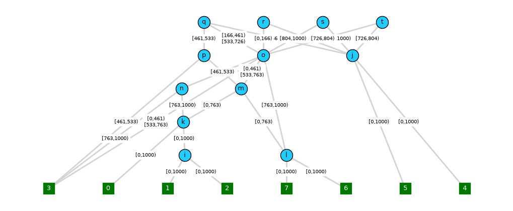
For more general graph plots, it can be helpful convert the tree sequence to a
networkx graph first, as described in the
Other graph analysis section of the ARGs as tree sequences tutorial.
This provides interfaces to graph plotting software such as
graphviz, which provides the dot layout engine for
directed graphs:
import networkx as nx
from IPython.display import SVG

def graphviz_svg(networkx_graph):
    AG = nx.drawing.nx_agraph.to_agraph(networkx_graph)  # Convert to graphviz "agraph"
    nodes_at_time_0 = [k for k, v in networkx_graph.nodes(data=True) if v['time'] == 0]
    AG.add_subgraph(nodes_at_time_0, rank='same')  # put time=0 at same rank
    return AG.draw(prog="dot", format="svg")

G = to_networkx_graph(ts, interval_lists=True)  # Function from the ARG tutorial
print("Converted `ts` to a networkx graph named `G`")
print("Plotting using graphviz...")
SVG(graphviz_svg(G))
Converted `ts` to a networkx graph named `G`
Plotting using graphviz...

Alternatively, you can read the graphviz positions back into networkx
and use the networkx drawing functionality, which
relies upon the matplotlib library. This
allows modification of node colours and symbols, labels, rotations,
annotations, etc., as shown below:
Note, however, that finding node and edge layout positions that avoid too much overlap can be tricky, even for the graphviz layout engine, and there is no easy functionality to place nodes at specific vertical (time) positions.
Demographic processes#
If you are generating a tree sequence via a Demes model, then you can visualize a schematic of the demography itself (rather than the resulting tree sequence) using the DemesDraw software. For example, here’s the plotting code to generate the demography plot from the “What is a tree sequence?” tutorial:

Geography#
Todo
How to get lat/long information out of a tree sequence and plot ancestors (or a tree) on a geographical landscape.