ARGs as tree sequences

At its heart, a tskit tree sequence consists of a list of Nodes, and a list of Edges that connect parent to child nodes. Therefore a succinct tree sequence is equivalent to a directed graph, which is additionally annotated with genomic positions such that at each position, a path through the edges exists which defines a tree. This graph interpretation of a tree sequence is tightly connected to the concept of an “ancestral recombination graph” (or ARG). See this preprint for further details.

Full ARGs

An original, narrower definition, which we do not use here, restricts the term ARG to the neutral coalescent process with simple crossover-recombination, and the graph structure defined by that process, see e.g. Griffiths & Marjoram (1997)

The term “ARG” is often used to refer to a structure consisting of nodes and edges that describe the genetic genealogy of a set of sampled chromosomes which have evolved via a process of genetic inheritance combined with recombination. ARGs may contain not just nodes corresponding to genetic coalescence, but also additional nodes that correspond e.g. to recombination events. These “full ARGs” can be stored and analysed in tskit like any other tree sequence. A full ARG can be generated using msprime.sim_ancestry() with the record_full_arg=True option, as described in the msprime docs:

import msprime

parameters = {
    "samples": 3, # Three diploid individuals == six sample genomes
    "sequence_length": 1e4,
    "recombination_rate": 1e-7,
    "population_size": 1e3,
    "random_seed": 333,
}

ts_arg = msprime.sim_ancestry(**parameters, record_full_arg=True, discrete_genome=False)
# NB: the strict Hudson ARG needs unique crossover positions (i.e. a continuous genome)

print('Simulated a "full ARG" under the Hudson model:')
print(
    f" ARG stored in a tree sequence with {ts_arg.num_nodes} nodes and"
    f" {ts_arg.num_edges} edges (creating {ts_arg.num_trees} local trees)"
)

Simulated a "full ARG" under the Hudson model:
 ARG stored in a tree sequence with 17 nodes and 18 edges (creating 3 local trees)

Like any tree sequence, we can also add mutations to the ARG to generate genetic variation:

import numpy as np
mu = 1e-7
ts_arg = msprime.sim_mutations(ts_arg, rate=mu, random_seed=888)
print("     Sample node:  " + "   ".join(str(u) for u in ts_arg.samples()))
for v in ts_arg.variants():
    print(f"Variable site {v.site.id}:", np.array(v.alleles)[v.genotypes])

     Sample node:  0   1   2   3   4   5
Variable site 0: ['T' 'C' 'T' 'C' 'C' 'C']
Variable site 1: ['C' 'C' 'C' 'C' 'G' 'C']
Variable site 2: ['T' 'T' 'G' 'T' 'T' 'T']

Visualization

In an msprime full ARG, recombinations are recorded in a specific way, by storing the parental genomes of a gamete. This means that two tskit nodes are created for each recombination, capturing transmission to the left vs right of the crossover breakpoint. These two nodes, which exist at the same timepoint, are identified by the NODE_IS_RE_EVENT and are displayed as a single point in the “ortho” viz below, labelled with two node IDs separated by a slash.

The normal Visualization of a tree sequence is as a set of local trees. However, all tree sequences can also be plotted as graphs. In particular, the Hudson “full ARG” model guarantees that the graph consists of nodes which mark a split into two child lineages (“common ancestor” nodes) or nodes which mark a split into two parent lineages (“recombination” nodes). Such ARGs can be visualized with edges drawn as horizontal and vertical lines (the “ortho” style in the tskit_arg_visualiser software):

Show code cell source Hide code cell source

%%javascript
require.config({paths: {d3: 'https://d3js.org/d3.v7.min'}});
require(["d3"], function(d3) {window.d3 = d3;});

import tskit_arg_visualizer
d3arg = tskit_arg_visualizer.D3ARG.from_ts(ts=ts_arg)
w, h = 450, 300  # width and height
d3arg.draw(w, h, edge_type="ortho", sample_order=[0, 2, 1, 3, 5, 4])

Local trees and arity

Below is a plot of the equivalent local trees in the ARG above, colouring recombination nodes in red and common ancestor nodes (unlabelled) in blue.

Show code cell source Hide code cell source

# Plot the recombination nodes in red, with a horizontal line at the time of occurrence,
# and only label nodes that are samples or recombination nodes.
samples = set(ts_arg.samples())
re_nodes = set(nd.id for nd in ts_arg.nodes() if nd.flags & msprime.NODE_IS_RE_EVENT)
ca_nodes = set(np.arange(ts_arg.num_nodes)) - re_nodes - samples
re_times = [int(nd.time) for nd in ts_arg.nodes() if nd.flags & msprime.NODE_IS_RE_EVENT]
style = ".y-axis .grid {stroke: #ff000033} .mut .sym {stroke: goldenrod}"
for u in re_nodes:
    style += f".n{u} > .sym {{fill: red}}"
for u in ca_nodes:
    style += f".n{u} > .sym {{fill: blue}}"
ts_arg.draw_svg(
    size=(600, 300),
    y_axis=True,
    y_ticks=re_times,
    y_gridlines=True,
    style=style,
    mutation_labels={},
    node_labels={u: u for u in samples | re_nodes}
)

The number of children descending from a node in a local tree can be termed the “local arity” of that node. It is clear from the plot above that red nodes always have a local arity of 1, and blue nodes sometimes do. This may seem an unusual state of affairs: tree representations often focus on branch-points, and ignore nodes with a single child. Indeed, it is possible to simplify the ARG above, resulting in a graph whose local trees only contain branch points or tips (i.e. local arity is never 1). Such a graph is more compact than the full ARG, but it omits some information about the timings and topological operations associated with recombination events and some common ancestor events. This information, as captured by the local unary nodes, is useful for

1. Retaining precise information about the time and lineages involved in recombination. This is required e.g. to ensure we can always work out the tree editing (or subtree-prune-and-regraft (SPR)) moves required to change one local tree into another as you move along the genome.

2. Calculating the likelihood of an full ARG under a specific model of evolution (most commonly, the neutral coalescent with recombination, or CwR, as modelled e.g. by Hudson (1983))

SPRs and recombination

The location of the recombination nodes in the trees above imply that the recombination events happened ~588 and ~59 generations ago. The older one, at 588 generations, involved node 13 (to the left of position 2601.01) and node 14 (to the right). As well as narrowing down the recombination event to a specific point in time, the position of these two nodes tells us that the SPR to convert the first into the second tree involves pruning the branch above samples 1, 3, 4, and 5 and regrafting it onto the branch above samples 0 and 2, rather than the other way around. Note that this particular recombination does not change the topology of the tree, but simply the branch lengths.

The recombination event 59 generations ago involved nodes 7 and 8, with the crossover ocurring at position 6516.94. The SPR operation which converts the middle tree into the last one involves pruning the branch above sample node 5 and regrafting it onto the branch above the common ancestor of 1 and 3. In this case, the recombination has led to a change in topology, such that the closest relative of 5 is node 4 from positions 0 to 6516.94, but 1 and 3 from positions 6516.94 to 10,000.

Calculating likelihoods

Because our ARG above was generated under the standard Hudson model (e.g. neutral evolution in a large population with unique recombination breakpoints along a continuous genome), we can calculate its likelihood under that model, for a given recombination rate and population size, using the msprime.log_arg_likelihood() method:

print(
    "Log likelihood of the genealogy under the Hudson model:",
    msprime.log_arg_likelihood(
        ts_arg,
        recombination_rate=parameters["recombination_rate"],
        Ne=parameters["population_size"]
    )
)

Log likelihood of the genealogy under the Hudson model: -89.68606886284756

Note

This likelihood calculation is tied to the specific tskit representation of the ARG that is output by the msprime simulator. In particular, it expects each recombination event to correspond to two recombination nodes, which allows so-called “diamond” events to be represented, in which both parents at a recombination event trace directly back to the same common ancestor.

Simplification

If we fully simplify the tree above, all remaining nodes (apart from the samples) will have a local arity greater than one. This loses information about the timings of recombination and non-coalescent common ancestry, but it still keeps the local tree structure intact:

ts = ts_arg.simplify()
ts.draw_svg(
    size=(600, 300),
    y_axis=True,
    node_labels={u: u for u in ts.samples()},
    mutation_labels={},
    style=".mut .sym {stroke: goldenrod}",
    y_ticks=[t*500 for t in range(4)]
)

Note that all recombination nodes have been lost from this graph; the effects of recombination are instead reflected in more recent coalescent nodes that are recombinant decendants of the original recombination nodes. This results in graph nodes which simultanousely have multiple children and multiple parents. Graphs with such nodes are unsuited to the “ortho” style of graph plotting. Instead, we can plot the tree sequence graph using diagonal lines:

d3graph = tskit_arg_visualizer.D3ARG.from_ts(ts=ts)
d3graph.draw(w, h, sample_order=[0, 2, 1, 3, 5, 4])

These “simplified” graphs are what are produced as the default msprime output. The exact SPR moves from tree to tree may no longer be obvious, and the ARG likelihood cannot be calculated from a tree sequence of this form.

Note that we can still calculate the mutation likelihood (i.e. the likelihood of the observed pattern of mutations, given the genealogy) because the topology and branch lengths of the local trees remain unchanged after simplification:

print("Log likelihood of mutations given the genealogy:")
print(' "full" ARG:',  msprime.log_mutation_likelihood(ts_arg, mutation_rate=mu))
print(" simplified:", msprime.log_mutation_likelihood(ts, mutation_rate=mu))

Log likelihood of mutations given the genealogy:
 "full" ARG: -33.204860594400216
 simplified: -33.204860594400216

Disadvantages of Full ARGs

There are two main reasons why you might not want to store a full ARG, but instead use a simplified version. Firstly if you are inferring ARGs from real data (rather than simulating them), it may not be possible or even desirable to infer recombination events. Often there are many possible recombination events which are compatible with a given set of recombined genome sequences.

Secondly, even if you are simulating genetic ancestry, storing full ARG requires many extra nodes. In fact, as the sequence length increases, the non-coalescent nodes come to dominate the tree sequence. We can calculate the percentage of non-coalescent nodes by comparing a full ARG with its simplified version:

large_sim_parameters = parameters.copy()
large_sim_parameters["sequence_length"] *= 1000
large_ts_arg = msprime.sim_ancestry(**large_sim_parameters, record_full_arg=True)
large_ts = large_ts_arg.simplify()

print(
    "Non-coalescent nodes take up "
    f"{(1-large_ts.num_nodes/large_ts_arg.num_nodes) * 100:0.2f}% "
    f"of this {large_ts.sequence_length/1e6:g} megabase {large_ts.num_samples}-tip ARG"
)

Non-coalescent nodes take up 99.32% of this 10 megabase 6-tip ARG

This is one of the primary reasons that nodes which are never associated with coalescent events are excluded by default in simulation software such as msprime and SLiM.

Note

As well as ancestrally relevant nodes, the original (mathematical) ARG formulation by Griffiths (1991) includes recombination nodes that are not ancestral to the samples. This leads to a graph with an vastly larger number of nodes than even the ARGs simulated here, and using such structures for simulation or inference is therefore infeasible.

ARG formats and tskit

It is worth noting a subtle and somewhat philosophical difference between some classical ARG formulations, and the ARG formulation used in tskit. Classically, nodes in an ARG are taken to represent events (specifically, “common ancestor”, “recombination”, and “sampling” events), and genomic regions of inheritance are encoded by storing a specific breakpoint location on each recombination node. In contrast, nodes in a tskit ARG correspond to genomes. More crucially, inherited regions are defined by intervals stored on edges (via the left and right properties), rather than on nodes. Here, for example, is the edge table from our ARG:

ts_arg.tables.edges

id	left	right	parent	child	metadata
0	0.00000000	10000.00000000	6	1
1	0.00000000	10000.00000000	6	3
2	0.00000000	6516.94017928	7	5
3	6516.94017928	10000.00000000	8	5
4	0.00000000	10000.00000000	9	6
5	6516.94017928	10000.00000000	9	8
6	0.00000000	10000.00000000	10	4
7	0.00000000	6516.94017928	10	7
8	0.00000000	10000.00000000	11	0
9	0.00000000	10000.00000000	11	2
10	0.00000000	10000.00000000	12	9
11	0.00000000	10000.00000000	12	10
12	0.00000000	2601.01454798	13	12
13	2601.01454798	10000.00000000	14	12
14	0.00000000	10000.00000000	15	11
15	2601.01454798	10000.00000000	15	14
16	0.00000000	2601.01454798	16	13
17	0.00000000	2601.01454798	16	15

Technically therefore, ARGs stored by tskit are edge-annotated “genome ARGs”, or gARGs. This flexible format can describe both simulated genetic ancestries (including those involving Gene conversion), and e.g. real-world genetic ancestries, such as inferrred recombining viral genealogies. The focus on genomes rather than events is also what makes simplification possible, and means tskit can encode ancestry without having to pin down exactly when specific ancestral events took place.

Working with ARGs in tskit

All tree sequences, including, but not limited to full ARGs, can be treated as directed (acyclic) graphs. Although many tree sequence operations operate from left to right along the genome, some are more naturally though of as passing from node to node via the edges, regardless of the genomic position of the edge. This section describes some of these fundamental graph operations.

Graph traversal

The standard edge iterator, TreeSequence.edge_diffs(), goes from left to right along the genome, matching the TreeSequence.trees() iterator. Although this will visit all the edges in the graph, these will not necessarily be grouped by the node ID either of the edge parent or the edge child. To do this, an alternative traversal (from top-to-bottom or bottom-to-top of the tree sequence) is required.

To traverse the graph by node ID, the TreeSequence.nodes() iterator can be used. In particular, because parents are required to be strictly older than their children, iterating through nodes using order="timeasc" will ensure that children are always visited before their parents (similar to a breadth-first or “level order” search). However, using TreeSequence.nodes() is inefficient if you also want to access the edges associated with each node.

The examples below show how to efficiently visit the all the edges in a tree sequence, grouped by the nodes to which they are connected, while also ensuring that children are visited before parents (or vice versa).

Traversing parent nodes

The most efficient graph traversal method visits all the parent nodes in the tree sequence, grouping edges for which that node is a parent. This is simple because edges in a tree sequence are ordered firstly by the time of the parent node, then by node ID.

import itertools
import operator
def edges_by_parent_timeasc(ts):
    return itertools.groupby(ts.edges(), operator.attrgetter("parent"))

for parent_id, edges in edges_by_parent_timeasc(ts):
    t = ts.node(parent_id).time
    children = {e.child for e in edges}
    print(f"Node {parent_id} at time {t} has these child node IDs: {children}")

Node 6 at time 56.0454802286223 has these child node IDs: {1, 3}
Node 7 at time 120.7850821708138 has these child node IDs: {5, 6}
Node 8 at time 142.86643656492956 has these child node IDs: {4, 5}
Node 9 at time 236.7237255340037 has these child node IDs: {0, 2}
Node 10 at time 272.05118690557765 has these child node IDs: {8, 4, 6, 7}
Node 11 at time 610.912738605865 has these child node IDs: {9, 10}
Node 12 at time 1382.4658244607965 has these child node IDs: {9, 10}

This visits children before parents. To visit parents before children, you can simply use reversed(ts.edges()) rather than ts.edges() within the groupby function. Note that terminal nodes (i.e. which are either isolated or leaf nodes in all local trees) are not visited by this function: therefore the method above will omit all the terminal sample nodes.

Traversing child nodes

Sometimes you may wish to iterate over all the edges for which a node is a child (rather than a parent). This can be done by sorting the edges by child node time (then child node id). This is a little slower, but can be done relatively efficiently as follows:

import itertools
import operator
import numpy as np
def edges_by_child_timeasc(ts):
    # edges sorted by child node time, then child node id using np.lexsort
    it = (ts.edge(u) for u in np.lexsort((ts.edges_child, ts.nodes_time[ts.edges_child])))
    return itertools.groupby(it, operator.attrgetter("child"))

for child_id, edges in edges_by_child_timeasc(ts):
    t = ts.node(child_id).time
    parents = {e.parent for e in edges}
    print(f"Node {child_id} at time {t} has these parent node IDs: {parents}")

Node 0 at time 0.0 has these parent node IDs: {9}
Node 1 at time 0.0 has these parent node IDs: {6}
Node 2 at time 0.0 has these parent node IDs: {9}
Node 3 at time 0.0 has these parent node IDs: {6}
Node 4 at time 0.0 has these parent node IDs: {8, 10}
Node 5 at time 0.0 has these parent node IDs: {8, 7}
Node 6 at time 56.0454802286223 has these parent node IDs: {10, 7}
Node 7 at time 120.7850821708138 has these parent node IDs: {10}
Node 8 at time 142.86643656492956 has these parent node IDs: {10}
Node 9 at time 236.7237255340037 has these parent node IDs: {11, 12}
Node 10 at time 272.05118690557765 has these parent node IDs: {11, 12}

To visit parents before children, the lexsort can take the negated -ts.nodes_time rather than simply using ts.nodes_time. Note that nodes which are never children of an edge are not visited by this algorithm. Such nodes are either isolated or a root in each local tree.

Other graph analysis

For graph-theory based analysis, it can be helpful to convert a tree sequence to a networkx graph. This can be done using the following code:

import tskit
import networkx as nx
import pandas as pd

def to_networkx_graph(ts, interval_lists=False):
    """
    Make an nx graph from a tree sequence. If `intervals_lists` is True, then
    each graph edge will have an ``intervals`` attribute containing a *list*
    of tskit.Intervals per parent/child combination. Otherwise each graph edge
    will correspond to a tskit edge, with a ``left`` and ``right`` attribute.
    """
    D = dict(source=ts.edges_parent, target=ts.edges_child, left=ts.edges_left, right=ts.edges_right)
    G = nx.from_pandas_edgelist(pd.DataFrame(D), edge_attr=True, create_using=nx.MultiDiGraph)
    if interval_lists:
        GG = nx.DiGraph()  # Mave a new graph with one edge that can contai
        for parent, children in G.adjacency():
            for child, edict in children.items():
                ilist = [tskit.Interval(v['left'], v['right']) for v in edict.values()]
                GG.add_edge(parent, child, intervals=ilist)
        G = GG
    nx.set_node_attributes(G, {n.id: {'flags':n.flags, 'time': n.time} for n in ts.nodes()})
    return G

arg = to_networkx_graph(ts_arg)

It is then possible to use the full range of networkx functions to analyse the graph:

assert nx.is_directed_acyclic_graph(arg)  # All ARGs should be DAGs
print("All descendants of node 10 are", nx.descendants(arg, 10))

All descendants of node 10 are {4, 5, 7}

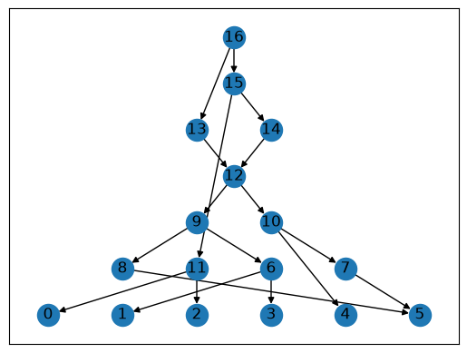
Networkx also has some built-in drawing functions: below is one of the simplest ones (for other possibilities, see the Visualization tutorial).

for layer, nodes in enumerate(nx.topological_generations(arg.reverse())):
    for node in nodes:
        arg.nodes[node]["layer"] = layer
pos = nx.multipartite_layout(arg, subset_key="layer", align='horizontal')

nx.draw_networkx(arg, pos=pos)

Other software

Todo

Show how ARGweaver output can be converted to tskit form.

Todo

Show how KwARG output can be converted to tskit form.

Todo

Implement conversion between the 2 RE node version and the 1 RE node version