Building a forward simulator

This tutorial shows how tskit can be used to build your own forward-time, tree sequence simulator from scratch. The simulator will use the discrete-time Wright-Fisher model, and track individuals along with their genomes, storing inherited genomic regions as well as the full pedigree.

The code in this tutorial is broken into separate functions for clarity and to make it easier to modify for your own purposes; a simpler and substantially condensed forward-simulator is coded as a single function at the top of the Completing forwards simulations tutorial.

Note

If you are simply trying to obtain a tree sequence which is the result of a forward-time simulation, this can be done by using one of the highly capable forward-time genetic simulators that already exist, such as SLiM or fwdpy11. Documentation and tutorials for these tools exist on their respective websites. This tutorial is instead intended to illustrate the general principles that lie behind such simulators.

We will focus on the case of diploids, in which each individual contains 2 genomes, but the concepts used here generalize to any ploidy, if you are willing to do the book-keeping. The individuals themselves are not strictly necessary for representing genetic genealogies (it’s the genomes which are important), but they are needed during the simulation, and so we record them in the resulting output for completeness.

Definitions

Before we can make any progress, we require a few definitions.

A node represents a genome at a point in time (often we imagine this as the “birth time” of the genome). It can be described by a tuple, (id, time), where id is a unique integer, and time reflects the birth time of that id. When generating a tree sequence, this will be stored in a row of the Node Table.

A diploid individual is a group of two nodes. During simulation, a simple and efficient grouping assigns sequential pairs of node IDs to an individual. It can be helpful (but not strictly necessary) to store individuals within the tree sequence as rows of the the Individual Table (a node can then be assigned to an individual by storing that individual’s id in the appropriate row of the node table).

An edge reflects a transmission event between nodes. An edge is a tuple (Left, Right, Parent, Child) whose meaning is “The Child genome inherited the genomic interval [Left, Right) from the Parent genome”. In a tree sequence this is stored in a row of the Edge Table.

The time, in the discrete-time Wright-Fisher (WF) model which we will simulate, is measured in integer generations. To match the tskit notion of time, we record time in generations ago: i.e. for a simple simulation of G generations, we start the simulation at generation \(G-1\) and count down until we reach generation 0 (the current-day).

The population consists of \(N\) diploid individuals (\(2N\) nodes) at a particular time \(t\). At the start, the population will have no known ancestry, but subsequently each individual will be formed by choosing (at random) two parent individuals from the population in the previous generation.

Approach

We will generate edges, nodes, and individuals forwards in time, adding them to the relevant tskit tables. To aid efficiency, we will also see how to “simplify” the tables into the minimal set of nodes and edges that describe the history of the sample. Finally, these tables can be exported into an immutable TreeSequence for storing or analysis.

Setup

First, we’ll import the necessary libraries and define some general parameters. The numpy library will be used to produce random numbers.

import tskit
import numpy as np

random_seed = 2
random = np.random.default_rng(random_seed)  # A random number generator for general use

L = 50_000  # The sequence length: 50 Kb

Core steps

The core simulation function generates a new population by repeating the following steps:

1. Pick a pair of parent individuals at random from the population in the previous generation.

2. Create a new child individual with two genomes (an individual ID will be created by adding a row to the individual table and two nodes IDs will be created by adding two rows to the node table. If desired, we can also provide the parent IDs when adding to the individual table, which will result in storing the entire genealogical pedigree.

3. Add the inheritance paths for each child genome using an add_inheritance_paths() function (defined later).

We will also define a simpler function, involving just step 2, to create the initial population.

For convenience, the population will be stored in a Python dictionary that maps the individual ID to the IDs of its two genomes. Note that in lower-level languages such as C, rather than use a mapping of individual ID to two genomes, we could instead rely on the fact that genome IDs are allocated sequentially, and pick a random pair of genomes from the previous population directly, without using individual IDs.

# For visualising unsimplified tree sequences, it can help to flag all nodes as samples
default_node_flags = tskit.NODE_IS_SAMPLE

def make_diploid(tables, time, parent_individuals=None) -> tuple[int, tuple[int, int]]:
    """
    Make an individual and its diploid genomes by adding to tables, returning the IDs.
    Specifying parent_individuals is optional but results in the pedigree being stored.
    """
    individual_id = tables.individuals.add_row(parents=parent_individuals)
    return individual_id, (
        tables.nodes.add_row(default_node_flags, time, individual=individual_id),
        tables.nodes.add_row(default_node_flags, time, individual=individual_id),
    )

def new_population(tables, time, prev_pop, recombination_rate) -> dict[int, tuple[int, int]]:
    pop = {}  # fill with individual_ID: (maternal_genome_ID, paternal_genome_ID)

    # Cache the list of individual IDs in the previous population, for efficiency
    prev_individuals = np.array([i for i in prev_pop.keys()], dtype=np.int32)

    for _ in range(len(prev_pop)):
        # 1. Pick two individual parent IDs at random, `replace=True` allows selfing
        mother_and_father = random.choice(prev_individuals, 2, replace=True)

        # 2. Get 1 new individual ID + 2 new node IDs
        child_id, child_genomes = make_diploid(tables, time, mother_and_father)
        pop[child_id] = child_genomes  # store the genome IDs
        
        # 3. Add inheritance paths to both child genomes
        for child_genome, parent_individual in zip(child_genomes, mother_and_father):
            parent_genomes = prev_pop[parent_individual]
            add_inheritance_paths(tables, parent_genomes, child_genome, recombination_rate)
    return pop

def initialise_population(tables, time, size) -> dict[int, tuple[int, int]]:
    # Just return a dictionary by repeating step 2 above
    return dict(make_diploid(tables, time) for _ in range(size))

Note

For simplicity, the code above assumes any parent can be a mother or a father (i.e. this is a hermaphrodite species). It also allows the same parent to be chosen as a mother and as a father (i.e. “selfing” is allowed), which gives simpler theoretical results. This is easy to change if required.

Our forward-time simulator simply involves repeatedly running the next_population() routine, replacing the old population with the new one. For efficiency reasons, tskit has strict requirements for the order of edges in the edge table, so we need to sort() the tables before we output the final tree sequence.

def forward_WF(num_diploids, seq_len, generations, recombination_rate=0, random_seed=2):
    """
    Run a forward-time Wright Fisher simulation of a diploid population, returning
    a tree sequence representing the genetic genealogy of the simulated genomes.
    """
    global random
    random = np.random.default_rng(random_seed) 
    tables = tskit.TableCollection(seq_len)
    tables.time_units = "generations"  # optional, but helpful when plotting

    pop = initialise_population(tables, generations, num_diploids)
    while generations > 0:
        generations = generations - 1
        pop = new_population(tables, generations, pop, recombination_rate)

    tables.sort()
    return tables.tree_sequence()

Inheritance without recombination

The final piece of the simulation is to define the add_inheritance_paths() function, which saves the inheritance paths in the Edge Table. For reference, the simplest case (a small focal region in which there is no recombination) can be coded as follows:

def add_inheritance_paths(tables, parent_nodes, child_node, recombination_rate):
    "Add inheritance paths from a randomly chosen parent genome to the child genome."
    assert recombination_rate == 0
    left, right = [20_000, 21_000]  # only define inheritance in this focal region
    inherit_from = random.integers(2)  # randomly choose the 1st or the 2nd parent node
    tables.edges.add_row(left, right, parent_nodes[inherit_from], child_node)

Inheritance with recombination

Recombination adds complexity to the inheritance paths from a child to its parents, that the child inherits a mosaic of the two genomes present in each parent.

The exact details of the mosaic will depend on the model of recombination you wish to implement. For instance, a simple model such as that in the Completing forwards simulations tutorial might assume exactly one crossover per chromosome. A complex model might allow not just multiple crossovers with e.g. recombination “hotspots”, but also non-crossover events such as Gene conversion.

Below is a redefined add_inheritance_paths() function of intermediate complexity, which models recombination as a uniform Poisson process along a genomic interval. We generate a set of “breakpoints” along the genome, then allocates edges from the child genome to one or the other genome from the parent, with left and right positions reflecting the breakpoint positions. Note that real recombination rates are usually such that they result in relatively few breakpoints per chromosome (in humans, around 1 or 2).

def add_inheritance_paths(tables, parent_genomes, child_genome, recombination_rate):
    "Add paths from parent genomes to the child genome, with crossover recombination."
    L = tables.sequence_length
    num_recombinations = random.poisson(recombination_rate * L)
    breakpoints = random.uniform(0, L, size=num_recombinations)
    breakpoints = np.concatenate(([0], np.unique(breakpoints), [L]))
    inherit_from = random.integers(2)  # starting parental genome

    # iterate over pairs of ([0, b1], [b1, b2], [b2, b3], ... [bN, L])
    for left, right in zip(breakpoints[:-1], breakpoints[1:]):
        tables.edges.add_row(
            left, right, parent_genomes[inherit_from], child_genome)
        inherit_from = 1 - inherit_from  # switch to other parent genome

Note

Above, breakpoint positions occur on a continuous line (i.e. “infinite breakpoint positions”), to match population genetic theory. It is relatively easy to alter this to allow recombinations only at integer positions

Basic examples

Now we can test the forward_WF() function for a single generation with a small population size of 6 diploids, and print out the resulting tree sequence. For simplicity, we will omit recombination for now.

ts = forward_WF(6, L, generations=1)
ts.draw_svg(y_axis=True, size=(500, 200))

It looks like it is working correctly: all 12 genomes (6 diploids) in the current generation at time=0 trace back to a genome in the initial generation at time=1. Note that not all individuals in the initial generation have passed on genetic material at this genomic position (they appear as isolated nodes at the top of the plot).

Now let’s simulate for a longer time period, and set a few helpful plotting parameters.

Note

By convention we plot the most recent generation at the bottom of the plot (i.e. perversely, each “tree” has leaves towards the bottom, and roots at the top)

ts = forward_WF(6, L, generations=20)

graphics_params = {
    "y_axis": True,
    "y_label": f"Time ({ts.time_units} ago)",
    "y_ticks": {i: 'Current' if i==0 else str(i) for i in range(21)},
}
ts.draw_svg(size=(1200, 400), **graphics_params)

This is starting to look like a real genealogy! Clearly, however, there are many “extinct” lineages that have not made it to the current day.

Simplification

The key to efficent forward-time genealogical simulation is the process of Simplification, which can reduce much of the complexity shown in the tree above. Typically, we want to remove all the lineages that do not contribute to the current day genomes. We do this via the simplify() method, specifying that only the nodes in the current generation are “samples”.

current_day_genomes = ts.samples(time=0)
simplified_ts = ts.simplify(current_day_genomes, keep_unary=True, filter_nodes=False)
simplified_ts.draw_svg(size=(600, 400), **graphics_params)

ID changes

We just simplified with filter_nodes=False, meaning that the tree sequence retained all nodes even after simplification, even those that are no longer part of the genealogy. By default (if filter_nodes is not specified), these nodes are removed, which changes the node IDs.

simplified_ts = ts.simplify(current_day_genomes, keep_unary=True)
simplified_ts.draw_svg(size=(600, 300), **graphics_params)

You can see that the list of nodes passed to simplify() (i.e. the current-day genomes) have become the first nodes in the table, numbered from 0..11; the remaining (internal) nodes have been renumbered from youngest to oldest.

Removing intermediate nodes

The keep_unary=True parameter meant that we kept intermediate (“unary”) nodes, even those that do not not represent branch-points in the tree. Often these are also unneeded, and by default we remove those too, although this will mean that we lose track of the pedigree of the individuals (which is stored in the parents column of the Individual Table). Since we are removing more nodes, the node IDs of non-samples will again change.

simplified_ts = ts.simplify(current_day_genomes)
simplified_ts.draw_svg(size=(400, 300), y_axis=True)

This is now looking much more like a “normal” genetic genealogy (a “gene tree”), in which all the sample genomes trace back to a single common ancestor.

Recombination

If we pass a non-zero recombination rate to the forward_WF() function, different regions of the genome may have different ancestries. This results in multiple trees along the genome.

rho = 1e-7
ts = forward_WF(6, L, generations=50, recombination_rate=rho)
print(f"A recombination rate of {rho} has created {ts.num_trees} trees over {ts.sequence_length} bp")

A recombination rate of 1e-07 has created 4 trees over 50000.0 bp

Here’s how the full (unsimplified) genealogy looks (labels omitted for clarity):

graphics_params["y_ticks"] = [0, 10, 20, 30, 40 ,50]
ts.draw_svg(size=(1000, 400), node_labels={}, symbol_size=2, **graphics_params)

Because we are showing the extinct lineages and the recombinations associated with them, this plot has many trees and nodes, and is rather confusing. However, Simplification can be equally applied to a recombinant genealogy, and will reduce the genealogy to something more managable for analysis and visualization.

ts = forward_WF(6, L, generations=100, recombination_rate=rho)
simplified_ts = ts.simplify(ts.samples(time=0))
graphics_params["y_ticks"] = [0, 10, 20, 30, 40 ,50]
simplified_ts.draw_svg(size=(1000, 300), **graphics_params)

Larger simulations

So far we have only simulated a relatively small population size (12 genomes / 6 diploids) for a short time. We can easily simulate for longer times, and increase the population size. In this case, simplification can have a dramatic effect on the disk storage and memory required:

from datetime import datetime

population_size = 100
gens = 1000  # ten times the population size
L = 500_000  # ten times the sequence length

start = datetime.now()
large_ts = forward_WF(population_size, L, gens, recombination_rate=rho)
print(
    f"Simulated {population_size} individuals ({population_size * 2} genomes)",
    f"for {gens} generations in {(datetime.now() - start).seconds:.1f} seconds",
)

Simulated 100 individuals (200 genomes) for 1000 generations in 7.0 seconds

print(f"Full tree sequence including dead lineages: {large_ts.nbytes/1024/1024:.2f} MB")
current_day_genomes = large_ts.samples(time=0)
simplified_ts = large_ts.simplify(current_day_genomes, keep_input_roots=True)
print(
    f"Tree sequence of current-day individuals: {simplified_ts.nbytes/1024/1024:.2f} MB,",
    f"{simplified_ts.num_trees} trees."
)
print(
    "Simplification has reduced the size by a factor of",
    f"{large_ts.nbytes / simplified_ts.nbytes:.2f}"
)

Full tree sequence including dead lineages: 16.79 MB
Tree sequence of current-day individuals: 0.05 MB, 113 trees.
Simplification has reduced the size by a factor of 320.58

The most obvious improvement when simulating genealogies in forward time is therefore to carry out regular simplification steps during the simulation, rather than just at the end. This is described in the next tutorial:

Ensuring coalescence

Even though the simulation above was run for hundreds of generations, there are still trees with multiple roots in some regions of the genome. 1000 generations is not therefore long enough to capture the ancestry back to a single common ancestor (i.e. to ensure “full coalescence” of all local trees):

from matplotlib import pyplot as plt
plt.figure(figsize=(7, 2))
plt.stairs(
    [tree.num_roots for tree in simplified_ts.trees()],
    simplified_ts.breakpoints(as_array=True),
    baseline=None,
)
plt.xlabel("Genome position (bp)")
plt.ylabel("Number of roots")
plt.show()

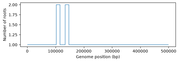
Most of our trees have one root, but a handful have two. What is happening is that even though we simulated for \(10N\) generations, and the theoretical expectation for the time to the most recent common ancestor is \(E[tMRCA]=4N\), the variance is pretty big, such that some marginal trees are not completely coalesced. Let’s take a look at the distribution of tMRCAs using msprime to carry out an equivalent backward-time simulation (which is much faster, so we can replicate it, say, 1000 times).

import msprime

tmrca=[]
sequence_length = 50_000
rho = 5e-7
for sim in msprime.sim_ancestry(
    100,
    sequence_length=sequence_length,
    recombination_rate=rho,
    random_seed=42,
    num_replicates=1000,
):
    for tree in sim.trees():
        tmrca.append(tree.time(tree.root))

plt.figure(figsize=(7, 3))
plt.hist(tmrca, bins=30, density=True)
plt.xlabel("tMRCA (units of N generations)")
plt.ylabel("Proportion of trees")
plt.show()

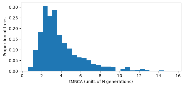
So, some fraction of local trees have very large tMRCAs! And of course the larger the population, the longer the time needed to ensure full coalescence. Hence for large forward simulation models, the number of generations required to ensure full coalescence can be prohibitive.

Uncoalesced local trees matter, because they result in some pairs of samples which are not connected, and so the genetic distance betweem them is undefined (another way to imagine this is that we cannot spot mutations that occur above the local roots of the tree). Hence the simulation is not capturing the full genetic diversity within the sample.

A powerful way to get around this problem is recapitation, in which an alternative technique, such as backward-in-time coalescent simulation, is used to to fill in the “head” of the tree sequence. In other words, we can use a fast backward-time simulator such as msprime to simulate the prior genealogy of the oldest nodes in the simplified tree sequence. Details are described in the Completing forwards simulations tutorial.

More complex forward-simulations

The next tutorial shows the principles behind more complex simulations, including e.g. regular simplification during the simulation, adding mutations, and adding metadata. It also details several extra tips and tricks we have learned when building forward simulators.