Quick start#
This page provides a quick overview of tstrait. We will be using sim_phenotype() to
demonstrate how quantitative traits can be simulated in tstrait.
To work with the examples, you will need to install msprime and matplotlib in addition to tstrait.
Learning Objectives
After this quick start page, you will be able to:
Understand how to simulate quantitative traits in tstrait
Understand how to read the output of tstrait
Input#
The main objective of tstrait is to simulate quantitative traits from a tree sequence input. The important
inputs of sim_phenotype() are:
- ts
The tree-sequence input with mutation
- num_causal
Number of causal sites
- model
The trait model where the effect sizes are going to be simulated
- h2
Narrow-sense heritability
Example#
import tstrait
import msprime

ts = msprime.sim_ancestry(
    samples=10_000,
    recombination_rate=1e-8,
    sequence_length=100_000,
    population_size=10_000,
    random_seed=100,
)
ts = msprime.sim_mutations(ts, rate=1e-8, random_seed=101)
ts.num_individuals
10000
Here, we have simulated a sample tree sequence with 10,000 individuals in msprime.
We will be using it in sim_phenotype() to simulate quantitative traits.
model = tstrait.trait_model(distribution="normal", mean=0, var=1)
sim_result = tstrait.sim_phenotype(
    ts=ts, num_causal=100, model=model, h2=0.3, random_seed=1
)
The sim_result variable created above contains simulated information of phenotypes and traits,
which will be shown below.
Trait Dataframe#
Simulated traits from sim_phenotype() can be extracted through .trait.
trait_df = sim_result.trait
trait_df.head()
| position | site_id | effect_size | causal_allele | allele_freq | trait_id | |
|---|---|---|---|---|---|---|
| 0 | 736 | 7 | 0.332814 | C | 0.00005 | 0 |
| 1 | 1901 | 10 | -0.651281 | T | 0.00035 | 0 |
| 2 | 2424 | 12 | 0.862445 | C | 0.00225 | 0 |
| 3 | 3095 | 17 | -0.125592 | T | 0.49985 | 0 |
| 4 | 4999 | 24 | 0.669153 | T | 0.00015 | 0 |
The trait_df is a pandas.DataFrame object that includes the following 6 columns:
position: Position of sites that have causal allele in genome coordinates.
site_id: Site IDs that have causal allele.
effect_size: Simulated effect size of causal allele.
causal_allele: Causal allele.
allele_freq: Allele frequency of causal allele.
trait_id: Trait ID that will be used in multi-trait simulation (See Multi-trait simulation for details).
Phenotype Output#
Simulated phenotypes from sim_phenotype() can be extracted through .phenotype.
phenotype_df = sim_result.phenotype
phenotype_df.head()
| trait_id | individual_id | genetic_value | environmental_noise | phenotype | |
|---|---|---|---|---|---|
| 0 | 0 | 0 | 7.013984 | 1.782352 | 8.796336 |
| 1 | 0 | 1 | 9.072514 | 4.237500 | 13.310014 |
| 2 | 0 | 2 | 4.096638 | 1.704231 | 5.800869 |
| 3 | 0 | 3 | 4.860104 | -6.721040 | -1.860936 |
| 4 | 0 | 4 | 6.569804 | 4.669378 | 11.239182 |
The phenotype_df is a pandas.DataFrame object that includes the following 5 columns:
trait_id: Trait ID and will be used in multi-trait simulation.
individual_id: Individual ID inside the tree sequence input.
genetic_value: Genetic value of individuals.
environmental_noise: Simulated environmental noise of individuals.
phenotype: Simulated phenotype, and it is a sum of genetic_value and environmental_noise.
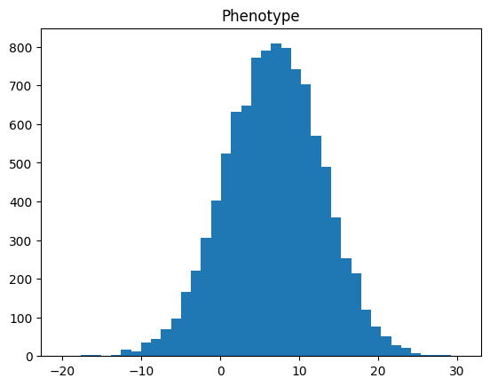
Next, we will be showing the distribution of simulated phenotype and environmental noise by creating
a histogram through using matplotlib.
import matplotlib.pyplot as plt
plt.hist(phenotype_df["phenotype"], bins=40)
plt.title("Phenotype")
plt.show()
plt.hist(phenotype_df["environmental_noise"], bins=40)
plt.title("Environmental Noise")
plt.show()
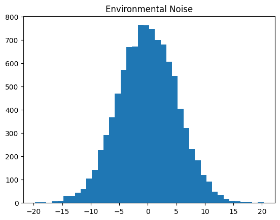
The environmental noise in tstrait follows a normal distribution. Please see Phenotype Model for mathematical details on the phenotype model and Effect Size Distribution for details on specifying the effect size distribution.
Normalise Phenotype#
The simulated phenotypes can be scaled by using the normalise_phenotypes() function. The function
will first normalise the phenotype by subtracting the mean of the input phenotype from each
value and divide it by the standard devitation of the input phenotype.
Afterwards, it scales the normalised phenotype based on the mean and variance input.
The output of normalise_phenotypes() is a pandas.DataFrame object with the scaled phenotypes.
An example usage of this function is shown below:
mean = 0
var = 1
normalised_df = tstrait.normalise_phenotypes(phenotype_df, mean=mean, var=var)
normalised_df.head()
| individual_id | trait_id | phenotype | |
|---|---|---|---|
| 0 | 0 | 0 | 0.333531 |
| 1 | 1 | 0 | 1.067976 |
| 2 | 2 | 0 | -0.153878 |
| 3 | 3 | 0 | -1.400572 |
| 4 | 4 | 0 | 0.731019 |
We see that the mean and variance of the normalised phenotype are 0 and 1, as we have indicated them
as inputs of normalise_phenotypes().
print("Mean of the normalised phenotype:", mean)
print("Variance of the normalised phenotype:", var)
Mean of the normalised phenotype: 0
Variance of the normalised phenotype: 1
The distribution of the normalised phenotype is shown below.
plt.hist(normalised_df["phenotype"], bins=40)
plt.title("Normalised Phenotype")
plt.show()
