Trait simulation#
This page describes how tstrait simulates traits and how to specify the effect size distribution.
Learning Objectives
After this effect size page, you will be able to:
Understand the mathematical details of the phenotype model in tstrait
Understand how to specify distributions of simulated effect sizes
Understand how to simulate effect size in tstrait and read its output
Understand how to simulate effect sizes from the frequency dependence architecture
Phenotype Model#
tstrait simulates a vector of quantitative trait \(y\) from the following additive model,
where \(X\) is the matrix that describes the number of causal alleles in each individual (the values in each row will be \(0\), \(1\), or \(2\) in the diploid setting, for example), \(\beta\) is the vector of effect sizes, and \(\epsilon\) is the vector of environmental noise. Environmental noise is simulated from the following distribution,
where \(V_G=Var(X\beta)\) and \(h^2\) is the narrow-sense heritability that is defined by the user.
The genetic values (\(X\beta\)) are obtained by simply adding up over all the genomes in each individual, regardless of ploidy.
See also
Genetic value for obtaining the genetic value \(X\beta\).
Environmental noise for simulating environmental noise \(\epsilon\).
Numericalisation of Genotypes for modifying the numericalisation of genotypes.
In this documentation, we will be describing how to simulate effect sizes in tstrait.
Effect Size Distribution#
The first step of trait simulation is to specify the distribution where the effect sizes will be
simulated. It can be specified in distribution input of trait_model(). We also specify
other parameters of the distribution in the function as well. For example,
import tstrait

model = tstrait.trait_model(distribution="normal", mean=0, var=1)
sets a trait model, where the effect sizes are simulated from a normal distribution with
mean \(0\) and variance \(1\). We can check the distribution name by using .name attribute
of a model instance.
model.name
'normal'
tstrait uses this distribution to simulate effect size \(\beta\) in the phenotype model described in (1).
The following effect size distributions are supported in tstrait, and please refer to links under Details for details on the input and distribution.
See also
Effect size distributions for details on the supported distributions.
Name |
Distribution |
Input |
Details |
|---|---|---|---|
|
Normal distribution |
|
|
|
Student’s t distribution |
|
|
|
Fixed value |
|
|
|
Exponential distribution |
|
|
|
Gamma distribution |
|
|
|
Multivariate normal distribution |
|
Effect Size Simulation#
Effect sizes can be simulated in tstrait by using tstrait.sim_trait(). In the example below,
we will be simulating effect sizes of 5 causal sites from a simulated tree sequence data in
msprime.
import msprime

ts = msprime.sim_ancestry(
    samples=10_000,
    recombination_rate=1e-8,
    sequence_length=100_000,
    population_size=10_000,
    random_seed=200,
)
ts = msprime.sim_mutations(ts, rate=1e-6, random_seed=200)

trait_df = tstrait.sim_trait(ts, num_causal=5, model=model, random_seed=1)
trait_df
| position | site_id | effect_size | causal_allele | allele_freq | trait_id | |
|---|---|---|---|---|---|---|
| 0 | 3440 | 1123 | -0.536953 | C | 0.00005 | 0 |
| 1 | 47072 | 15257 | 0.581118 | G | 0.00375 | 0 |
| 2 | 50840 | 16503 | 0.364572 | T | 0.00700 | 0 |
| 3 | 75539 | 24351 | 0.294132 | T | 0.00095 | 0 |
| 4 | 95010 | 30649 | 0.028422 | G | 0.00510 | 0 |
The trait dataframe has 6 columns:
position: Position of sites that have causal allele in genome coordinates.
site_id: Site IDs that have causal allele.
effect_size: Simulated effect size of causal allele.
causal_allele: Causal allele.
allele_freq: Allele frequency of causal allele.
trait_id: Trait ID that will be used in multi-trait simulation (See Multi-trait simulation for details).
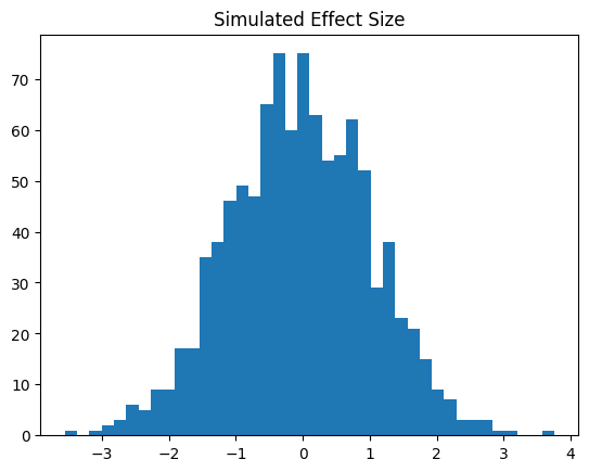
Next, we will be showing the distribution of simulated effect sizes by using a normal distribution trait model with 1,000 causal sites.
import matplotlib.pyplot as plt
model = tstrait.trait_model(distribution="normal", mean=0, var=1)
trait_df = tstrait.sim_trait(ts, num_causal=1000, model=model, random_seed=1)
trait_df.head()
plt.hist(trait_df["effect_size"], bins=40)
plt.title("Simulated Effect Size")
plt.show()

We see that the simulated effect sizes are approximately following a \(N(0,1)\) distribution, which coincides with the fact that we had specified a normal distribution trait model with mean 0 and variance 1.
Note
The site ID represents the IDs of causal sites, and information regarding the site can be
extracted by using .site().
The below code is used to extract information of site with ID 0 from ts tree sequence.
# Extract information of site with ID 0
ts.site(0)
Site(id=0, position=1.0, ancestral_state='C', mutations=[Mutation(id=0, site=0, node=40280, derived_state='T', parent=-1, metadata=b'', time=18036.72830221663, edge=41324, inherited_state='C')], metadata=b'')
The details of sites in tree sequences can be found here.
Frequency Dependence#
Tstrait supports frequency dependence simulation. It has been shown that rare variants
have increased effect sizes compared with common variants
Speed et al. (2017), so more realistic simulations
can be made possible by increasing the effect size on rarer variants. The alpha
parameter in sim_phenotype() and sim_trait() are used to control
the degree of frequency dependence on simulated effect sizes.
In the frequency dependence model, the following value is multiplied to the effect size:
In the above expression, \(p\) is the frequency of the causal allele, and
\(\alpha\) is the alpha input of sim_phenotype() and
sim_trait(). Putting a negative \(\alpha\) value increases the
magnitude of effect sizes on rare variants.
Note
The default alpha parameter in sim_phenotype() and
sim_trait() are 0, and frequency dependent model is not used. Please
ignore the alpha parameter if you are not interested in implementing the
frequency dependent model.
In the below example, we will be demonstrating how alpha influences the simulated
effect sizes by using a simulated tree sequence with 10,000 individuals.
ts = msprime.sim_ancestry(
    samples=10_000,
    recombination_rate=1e-8,
    sequence_length=1_000_000,
    population_size=10_000,
    random_seed=300,
)
ts = msprime.sim_mutations(ts, rate=1e-8, random_seed=303)
model = tstrait.trait_model(distribution="normal", mean=0, var=1)
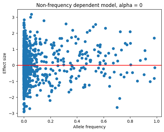
We will first simulate effect sizes by using the non-frequency dependent model
(alpha = 0), and visualize the simulated effect sizes. This is the default
alpha parameter in sim_trait(), so there is no need for you to specify
it in your trait simulation.
# trait.sim_trait(ts, num_causal=1000, model=model, random_seed=1)
# also works here
trait_df = tstrait.sim_trait(ts, num_causal=1000, model=model,
                             alpha=0, random_seed=1)

plt.scatter(trait_df.allele_freq, trait_df.effect_size)
plt.xlabel("Allele frequency")
plt.ylabel("Effect size")
plt.axhline(y=0, color='r', linestyle='-')
plt.title("Non-frequency dependent model, alpha = 0")
plt.show()

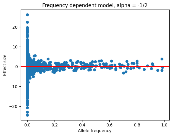
We see no relationship between allele frequency and effect size. As a next example,
we will be simulating effect sizes with alpha = -1/2.
trait_df = tstrait.sim_trait(ts, num_causal=1000, model=model,
                             alpha=-1/2, random_seed=1)

plt.scatter(trait_df.allele_freq, trait_df.effect_size)
plt.xlabel("Allele frequency")
plt.ylabel("Effect size")
plt.axhline(y=0, color='r', linestyle='-')
plt.title("Frequency dependent model, alpha = -1/2")
plt.show()

We see that rarer variants have increased effect sizes, as expected from the mathematical expression given in (2).
Specifying Causal Sites#
Instead of specifying the number of causal sites, users can directly provide the
causal sites as an input of sim_phenotype() and sim_trait().
When causal_sites argument of these functions are provided, tstrait will use
the inputted site IDs as causal sites, instead of randomly selecting causal
site IDs.
Example:
trait_df = tstrait.sim_trait(ts, causal_sites=[0, 3, 4], model=model,
                             alpha=-1/2, random_seed=1)
trait_df
| position | site_id | effect_size | causal_allele | allele_freq | trait_id | |
|---|---|---|---|---|---|---|
| 0 | 175 | 0 | 0.775715 | G | 0.02010 | 0 |
| 1 | 1567 | 3 | 2.634851 | A | 0.00475 | 0 |
| 2 | 1713 | 4 | 0.910507 | G | 0.00875 | 0 |