Multi-trait simulation

This page describes how to simulate multiple correlated traits in tstrait.

Learning Objectives

After this effect size page, you will be able to:

• Understand how multi-trait simulation is conducted in tstrait.

• Understand the trait models and inputs of multi-trait simulation.

Pleiotropy

tstrait supports simulation of multiple correlated traits, assuming that they are influenced by pleiotropic genes. Pleiotropy is used to describe the phenomenon that a single gene contributes to multiple traits (See here for details). The only trait model that is supported to simulate multiple traits in tstrait is multivariate normal distribution (TraitModelMultivariateNormal). We will be showing how to simulate traits by using a multivariate normal distribution trait model.

Multivariate normal distribution

The multivariate normal distribution trait model can be specified by inputting the mean vector and covariance matrix in trait_model(). Note that the covariance matrix must be symmetric and positive-semidefinite, and the dimensions of the mean vector and covariance matrix must match.

In the following example, we will be generating a multivariate normal distribution trait model with mean vector being a vector of zeros and covariance matrix being an identity matrix.

import tstrait
import numpy as np

model = tstrait.trait_model(
    distribution="multi_normal", mean=np.zeros(2), cov=np.eye(2)
)
model.num_trait

2

Note that 2 traits will be simulated from this model, as the dimension of the mean vector is 2.

Multi-trait simulation

We will now be simulating multiple traits by using a tree sequence data with 3 individuals and 2 causal sites.

import msprime

ts = msprime.sim_ancestry(
    samples=3,
    recombination_rate=1e-8,
    sequence_length=1_000_000,
    population_size=10_000,
    random_seed=5,
)
ts = msprime.sim_mutations(ts, rate=1e-8, random_seed=5)

sim_result = tstrait.sim_phenotype(
    ts=ts, num_causal=2, model=model, h2=[0.3, 0.3], random_seed=1
)

sim_result.phenotype

	trait_id	individual_id	genetic_value	environmental_noise	phenotype
0	0	0	0.905356	0.241850	1.147206
1	0	1	0.330437	0.574993	0.905430
2	0	2	0.000000	0.231250	0.231250
3	1	0	0.446375	-1.809578	-1.363203
4	1	1	-1.303157	1.257187	-0.045970
5	1	2	0.000000	0.619841	0.619841

sim_result.trait

	position	site_id	effect_size	causal_allele	allele_freq	trait_id
0	493419	474	0.330437	G	0.166667	0
1	493419	474	-1.303157	G	0.166667	1
2	523215	513	0.905356	G	0.166667	0
3	523215	513	0.446375	G	0.166667	1

Note

The dimension of narrow-sense heritability h2 must match the number of traits being simulated, and the multivariate normal distribution trait model can also be used as a model input of sim_trait() as well.

In the above example, phenotypic and effect size information of 2 traits are being simulated. The trait_id column represents the trait ID of the simulated traits.

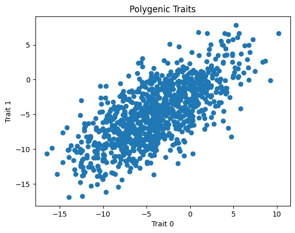
As a next example, we will be illustrating correlated quantitative traits by simulating correlated traits with 1000 causal sites and 1000 individuals.

ts = msprime.sim_ancestry(
    samples=1000,
    recombination_rate=1e-8,
    sequence_length=1_000_000,
    population_size=10_000,
    random_seed=5,
)
ts = msprime.sim_mutations(ts, rate=1e-8, random_seed=5)

cov = np.array([[1, 0.9], [0.9, 1]])

model = tstrait.trait_model(distribution="multi_normal", mean=np.zeros(2), cov=cov)

sim_result = tstrait.sim_phenotype(
    ts=ts, num_causal=100, model=model, h2=[0.8, 0.8], random_seed=1
)

We will be showing the correlation by creating a scatterplot in matplotlib.

import matplotlib.pyplot as plt

phenotype_df = sim_result.phenotype
trait0 = phenotype_df.loc[phenotype_df["trait_id"] == 0].phenotype
trait1 = phenotype_df.loc[phenotype_df["trait_id"] == 1].phenotype
plt.scatter(trait0, trait1)
plt.xlabel("Trait 0")
plt.ylabel("Trait 1")
plt.title("Polygenic Traits")
plt.show()