Working with traits and phenotypes#
An individual’s phenotype for a trait in SLiM is determined from that individual’s genetic effects, as well as both global and individual-specific “offsets”. SLiM records in metadata both phenotype and offset, so we can use these (by subtraction, for an additive trait) to determine the genetic value. We can also compute genetic contributions directly, which can be helpful, for instance, to decompose genetic variance from different parts of the genome.
Let’s start off with the simulation below, which has:
two additive traits,
with Gaussian selection on both,
started away from the optimum;
correlated mutational effects,
and also neutral mutations.
The recipe also saves the state of the population (by remembering everyone) every 5,000 generations. You may want to skip the details of the SLiM script on first reading: the simulation is more complex to display interesting trait dynamics. See the chapter on traits in the SLiM manual for more discussion, in particular the example “a model with two quantitative traits and pleiotropy”, from which this script was modified.
initialize() {
	setSeed(123);
	initializeTreeSeq();
	defineConstant("START1", -5.0);
	defineConstant("START2", 5.0);
	defineConstant("OPT1", 20.0);
	defineConstant("OPT2", -20.0);
	initializeTrait("trait1", "additive", baselineOffset=START1, individualOffsetSD=1.0);
	initializeTrait("trait2", "additive", baselineOffset=START2, individualOffsetSD=1.0);

	initializeMutationType("m1", NAN, "f", 0.0);   // neutral
	initializeMutationType("m2", NAN, "f", 0.0);   // QTLs
	m2.color = "red";
	m2.logMutationData(enable=T, effectSize=T);

	// g1 is a neutral region, g2 is a QTL
	initializeGenomicElementType("g1", m1, 1.0);
	initializeGenomicElementType("g2", c(m1,m2), c(1.0, 0.1));

	// chromosome of length 100 kb with two QTL regions
	initializeGenomicElement(g1, 0, 39999);
	initializeGenomicElement(g2, 40000, 49999);
	initializeGenomicElement(g1, 50000, 79999);
	initializeGenomicElement(g2, 80000, 89999);
	initializeGenomicElement(g1, 90000, 99999);
	initializeRecombinationRate(1e-8);
	initializeMutationRate(1e-7);

	// QTL-related constants used below
	defineConstant("QTL_mu", c(0.0, 0.0));
	defineConstant("QTL_cov", 0.25);
	defineConstant("QTL_sigma", matrix(c(1,QTL_cov,QTL_cov,1), nrow=2));
	}

1 late() {
	sim.addSubpop("p1", 500);
}

mutation(m2) {
	// draw mutational effects for the new m2 mutation
	effects = rmvnorm(1, QTL_mu, QTL_sigma);
	mut.setEffectSizeForTrait(NULL, effects);
	return T;
}

late() {
	sim.demandPhenotype(NULL, NULL);

	inds = sim.subpopulations.individuals;
	effects1 = 1.0 + dnorm(inds.trait1, OPT1, 15.0) * 10.0;
	effects2 = 1.0 + dnorm(inds.trait2, OPT2, 15.0) * 10.0;
	inds.fitnessScaling = effects1 * effects2;
}

1:1000000 late() {
	if (sim.cycle % 5000 == 1) {
		inds = p1.individuals;
		sim.treeSeqRememberIndividuals(inds);
		// keep running until we get close to both optima
		if ((abs(mean(inds.trait1) - OPT1) <= 1.0) & (abs(mean(inds.trait2) - OPT2) <= 1.0)) {
	   	sim.treeSeqOutput("phenotypes.trees", metadata=Dictionary("all_mutations", m2.loggedData("values")));
			sim.simulationFinished();
		}
	}
}
Trait distributions#
First, let’s load the result of the simulation and look at trait distributions in each of the saved time points.
ts = tskit.load("phenotypes.trees")
ts_metadata = ts.metadata
mut_metadata = pyslim.mutation_metadata(ts)
Here’s information about the traits:
ts_metadata['SLiM']['traits']
[{'baselineOffsetH': -5.0,
  'directFitnessEffect': False,
  'index': 0,
  'individualOffsetMean': 0.0,
  'individualOffsetSD': 1.0,
  'name': 'trait1',
  'substitutionAccumulation': True,
  'substitutionOffsetH': 24.79603424668312,
  'type': 'additive'},
 {'baselineOffsetH': 5.0,
  'directFitnessEffect': False,
  'index': 1,
  'individualOffsetMean': 0.0,
  'individualOffsetSD': 1.0,
  'name': 'trait2',
  'substitutionAccumulation': True,
  'substitutionOffsetH': -24.926677107810974,
  'type': 'additive'}]
The information matches the parameters passed to initializeTrait,
along with substitutionOffsetH, which we discuss below.
This is a simulation of hermaphrodites, so the baseline offsets we specified in script
(as START1 and START2 in the script)
are recorded here as baselineOffsetH. If this simulation had separate sexes,
there would be two baseline offsets: F and M.
Here’s the information we have about a given individual:
ts.individual(0)
Individual(id=0, flags=196608, location=array([0., 0., 0.]), parents=array([-1, -1], dtype=int32), nodes=array([7385, 7386], dtype=int32), metadata={
    'pedigree_id': 10000000,
    'pedigree_p1': 9999949,
    'pedigree_p2': 9999889,
    'tag': -9223372036854775808,
    'tagF': -1.7976931348623157e+308,
    'age': -1,
    'subpopulation': 1,
    'sex': -1,
    'tagL0_set': False,
    'tagL0': False,
    'tagL1_set': False,
    'tagL1': False,
    'tagL2_set': False,
    'tagL2': False,
    'tagL3_set': False,
    'tagL3': False,
    'tagL4_set': False,
    'tagL4': False,
    'per_trait': [{
        'phenotype': 19.158720654560593,
        'offset': -0.6373135921225269
       },
    {
     'phenotype': -19.82969840229935,
     'offset': 0.09697870551162334
    }]
   })
In particular, phenotype and offset values:
ts.individual(0).metadata['per_trait']
[{'phenotype': 19.158720654560593, 'offset': -0.6373135921225269},
 {'phenotype': -19.82969840229935, 'offset': 0.09697870551162334}]
Next, let’s find the birth time of each individual, and see which times we have information for (this is simple because it’s a WF simulation):
ind_times = ts.nodes_time[ts.individuals_nodes[:,0]]

from collections import Counter
Counter([int(t) for t in ind_times])
Counter({0: 500, 20000: 500, 15000: 500, 10000: 500, 5000: 500})
We can use the helpful metadata_vector method of table collections
to quickly pull out the phenotype and offset vectors:
num_traits = 2
ind_phenotypes = np.column_stack([
    ts.tables.individuals.metadata_vector(["per_trait", j, "phenotype"])
    for j in range(num_traits)
])
ind_offsets = np.column_stack([
    ts.tables.individuals.metadata_vector(["per_trait", j, "offset"])
    for j in range(num_traits)
])
For instance, here are the “phenotype” entries for the first five individuals (one column per trait):
ind_phenotypes[:5,:]
array([[ 19.15872065, -19.8296984 ],
       [ 21.34094365, -19.01111648],
       [ 20.08542214, -20.31883604],
       [ 17.52501805, -20.4797002 ],
       [ 20.3223109 , -18.45133827]])
To prepare to make the plots (using plotnine) we’ll put everything in a data frame:
df = pd.DataFrame({
    'pedigree_id' : ts.tables.individuals.metadata_vector("pedigree_id"),
    'time' : ind_times,
    "phenotype1" : ind_phenotypes[:,0],
    "offset1" : ind_offsets[:,0],
    "phenotype2" : ind_phenotypes[:,1],
    "offset2" : ind_offsets[:,1],
})
df.head()
| pedigree_id | time | phenotype1 | offset1 | phenotype2 | offset2 | |
|---|---|---|---|---|---|---|
| 0 | 10000000 | 0.0 | 19.158721 | -0.637314 | -19.829698 | 0.096979 |
| 1 | 10000001 | 0.0 | 21.340944 | 1.544909 | -19.011116 | 0.915561 |
| 2 | 10000002 | 0.0 | 20.085422 | 0.289388 | -20.318836 | -0.392159 |
| 3 | 10000003 | 0.0 | 17.525018 | -2.271016 | -20.479700 | -0.553023 |
| 4 | 10000004 | 0.0 | 20.322311 | 0.526277 | -18.451338 | 1.475339 |
Now, here’s phenotype distributions across these time slices. We can see that the population is moving from its initial position at (-5, 5) towards the optimum at (20, -20):
(
    df >> p9.ggplot(p9.aes(x="phenotype1", y="phenotype2", color="time"))
    + p9.geom_point()
)
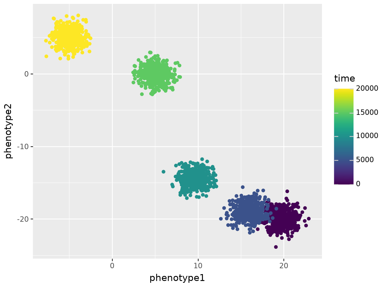
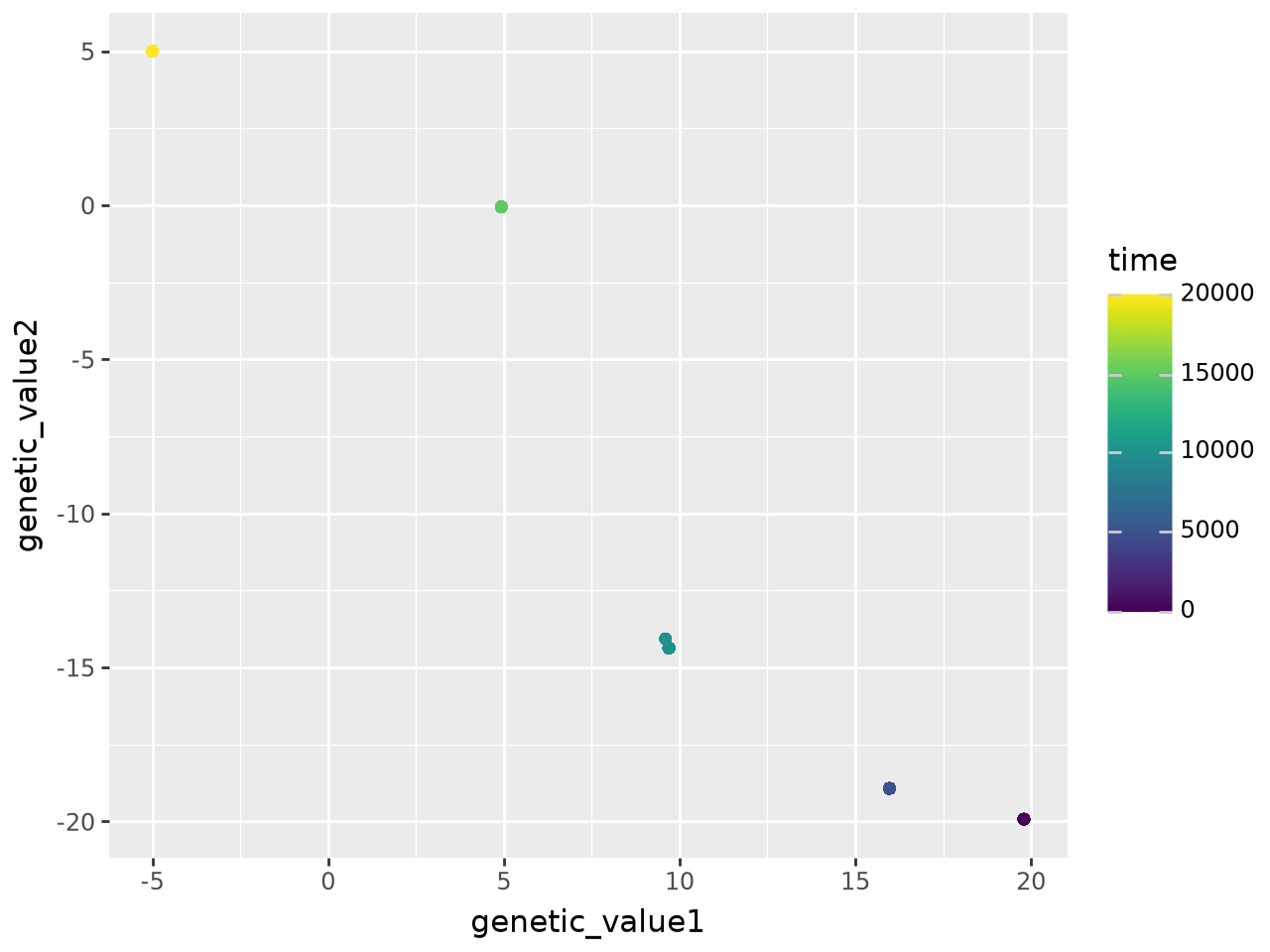
That’s the phenotypes; it turns out that most of that spread is actually “offset”, i.e., what’s usually called “environmental” noise. We can get the genetic contributions by subtracting the individual-level offsets:
df['genetic_value1'] = df['phenotype1'] - df['offset1']
df['genetic_value2'] = df['phenotype2'] - df['offset2']
Plotting these, we see the populations have very little genetic variation:
(
    df >> p9.ggplot(p9.aes(x="genetic_value1", y="genetic_value2", color="time"))
    + p9.geom_point()
)
Mutation effects#
Now let’s see how to use mutation information to calculate genetic values directly.
To do this, let’s take a simpler example.
This just has two additive traits, and mutations have independent effects on each trait.
Both traits are neutral, and so are only affected by drift and are not calculated at all
by SLiM until we call demandPhenotype.
There are two mutation types; the first is underdominant and the second is additive
(using the special NAN value for \(h\) to indicate independent dominance).
initialize() {
	setSeed(123);
	initializeTreeSeq(timeUnit="generations");
	initializeTrait("weight", "additive", baselineOffset=5.0, individualOffsetSD=0.2);
	initializeTrait("wing", "additive", baselineOffset=-1.0, individualOffsetSD=0.1);

	initializeMutationType("m1", 0.2, "n", 0.0, 0.01);
	initializeMutationType("m2", NAN, "n", 0.0, 0.01);

	initializeGenomicElementType("g1", c(m1,m2), c(0.5,0.5));

	initializeGenomicElement(g1, 0, 9999999);
	initializeRecombinationRate(1e-8);
	initializeMutationRate(1e-7);
}

1 late() {
	sim.addSubpop("p1", 50);
}

1000 late() {
	sim.demandPhenotype(NULL, NULL);
	sim.treeSeqOutput("phenotypes2.trees");
}
First, we load in the resulting tree sequence, and extract copies of top-level metadata and mutation metadata, as described in Mutation metadata:
ts = tskit.load("phenotypes2.trees")
ts_metadata = ts.metadata
mut_metadata = pyslim.mutation_metadata(ts)
Here’s the first mutation:
mut = ts.mutation(0)
mut
Mutation(id=0, site=0, node=116, derived_state='98288', parent=-1, metadata={
    'slim_ids': [98288]
   },
time=16.0, edge=261, inherited_state='')
We can see which SLiM mutation(s) this mutation represents
by looking up those SLiM mutation IDs in the mutation’s metadata:
mut.metadata["slim_ids"].
(As noted previously,
the same information is stored in mut.derived_state,
but we recommend pulling this information out of metadata.)
Then, we can find information about those SLiM mutations
in the top-level mutation metadata (here, mut_metadata,
obtained using mutation_metadata()).
mut_metadata[mut.metadata["slim_ids"][0]]
{'mutation_id': 98288,
 'mutation_type': 2,
 'subpopulation': 1,
 'slim_time': 984,
 'nucleotide': -1,
 'padding': None,
 'per_trait': [{'effect_size': -0.008490736596286297,
   'dominance': nan,
   'hemizygous_dominance': 1.0},
  {'effect_size': -4.386622822494246e-05,
   'dominance': nan,
   'hemizygous_dominance': 1.0}]}
So, we can use the effect_size and dominance
to calculate genetic effects (we won’t need hemizygous dominance,
since no-one is hemizygous in this simulation).
Here is a function that calculates the effect of a pair of alleles.
The function uses the derived_state property (a string) rather than the
metadata property because that’s what’s returned by tskit.TreeSequence.variants(),
which we’ll be using below.
from collections import Counter

def additive_effect(mut_metadata, a, b):
    # Here a and b are *string* derived states.
    num_traits = len(next(iter(mut_metadata.values()))['per_trait'])
    out = np.zeros((num_traits,))
    muts = Counter(a.split(",")) + Counter(b.split(","))
    for m in muts:
        if m != "":
            md = mut_metadata[int(m)]['per_trait']
            if muts[m] == 1:
                for j in range(num_traits):
                    h = md[j]['dominance']
                    if np.isnan(h):
                        h = 1/2
                    out[j] += 2 * md[j]['effect_size'] * h
            if muts[m] == 2:
                for j in range(num_traits):
                    out[j] += 2 * md[j]['effect_size']
    return out

# for instance, a homozygote for that mutation:
additive_effect(mut_metadata, mut.derived_state, mut.derived_state)
array([-1.69814732e-02, -8.77324564e-05])
Using this and tskit.TreeSequence.variants(),
we can compute genetic values for an individual:
def additive_genetic_value(ts, mut_metadata, ind):
    out = np.zeros((num_traits,))
    for v in ts.variants(samples=ind.nodes):
        x, y = [v.alleles[g] for g in v.genotypes]
        out += additive_effect(mut_metadata, x, y)
    return out

additive_genetic_value(ts, mut_metadata, ts.individual(0))
array([-0.11604283, -0.29277332])
The final component is offsets.
To match SLiM we need to add in both the individual’s offset
(which is stored in their metadata)
and the global (“baseline”) offset.
Within SLiM, the baselineOffsetX properties
(where X is F, M, or H) values are provided by the user
on initialization of the trait, and contribute to all individual’s phenotypes.
Within SLiM there is also the substitutionOffsetX property to consider,
but since the tree sequence does not distinguish substitutions from other mutations,
here we do nothing with these.
(For more on this, see the SLiM manual and Technical details.)
Here is a function that finds the offsets for an individual, depending on their sex, and combines them for an additive trait:
def additive_offset(ts_metadata, ind):
    k = {
        pyslim.INDIVIDUAL_TYPE_HERMAPHRODITE : "baselineOffsetH",
        pyslim.INDIVIDUAL_TYPE_FEMALE : "baselineOffsetF",
        pyslim.INDIVIDUAL_TYPE_MALE : "baselineOffsetM",
    }[ind.metadata["sex"]]
    out = np.array([x[k] for x in ts_metadata['SLiM']['traits']])
    out += [x['offset'] for x in ind.metadata['per_trait']]
    return out

additive_offset(ts.metadata, ts.individual(0))
array([ 4.83203513, -1.07860051])
Now we can compute phenotypes, and check they match what SLiM produced.
alive = pyslim.individuals_alive_at(ts, 0)
ind = ts.individual(alive[0])
print(f"Ours: {additive_genetic_value(ts, mut_metadata, ind) + additive_offset(ts_metadata, ind)}")
print(f"SLiM: {np.array([x['phenotype'] for x in ind.metadata['per_trait']])}")
Ours: [ 4.7159923  -1.37137383]
SLiM: [ 4.7159923  -1.37137383]
Happily, they match. Next we can compare for all individuals;
to actually check for equality we need to account for floating-point error,
since the numbers stored by SLiM and computed by us may differ by 1e-10 or so:
for ind in ts.individuals():
    our_pheno = additive_genetic_value(ts, mut_metadata, ind) + additive_offset(ts_metadata, ind)
    slim_pheno = np.array([x['phenotype'] for x in ind.metadata['per_trait']])
    assert np.allclose(our_pheno, slim_pheno)
Multiplicative and logistic traits#
To see how multiplicative and logistic traits work, we’ll change the first trait to be multiplicative and the second to be logistic:
initialize() {
	setSeed(123);
	initializeTreeSeq(timeUnit="generations");
	initializeTrait("mult", "multiplicative", baselineOffset=5.0, individualOffsetSD=0.1);
	initializeTrait("logistic", "logistic", baselineOffset=-1.0, individualOffsetSD=0.1);

	initializeMutationType("m1", 0.2, "n", 0.0, 0.01);
	initializeMutationType("m2", NAN, "n", 0.0, 0.01);

	initializeGenomicElementType("g1", c(m1,m2), c(0.5,0.5));

	initializeGenomicElement(g1, 0, 9999999);
	initializeRecombinationRate(1e-8);
	initializeMutationRate(1e-7);
}

1 late() {
	sim.addSubpop("p1", 50);
}

1000 late() {
	sim.demandPhenotype(NULL, NULL);
	sim.treeSeqOutput("phenotypes3.trees");
}
First, we load the information,
remembering to re-compute ts_metadata and mut_metadata:
ts = tskit.load("phenotypes3.trees")
ts_metadata = ts.metadata
mut_metadata = pyslim.mutation_metadata(ts)
Just for the heck of it, we’ll load the individual information into a data frame row-wise instead of column-wise:
df = pd.DataFrame([
        (
         ts.node(ind.nodes[0]).time,
         ind.metadata['per_trait'][0]['phenotype'],
         ind.metadata['per_trait'][0]['offset'],
         ind.metadata['per_trait'][1]['phenotype'],
         ind.metadata['per_trait'][1]['offset'],
        )
        for ind in ts.individuals()
    ],
    columns=['time', "phenotype1", "offset1", "phenotype2", "offset2"],
)
df.head()
| time | phenotype1 | offset1 | phenotype2 | offset2 | |
|---|---|---|---|---|---|
| 0 | 0.0 | 4.118879 | 0.919447 | 0.202398 | -0.078601 |
| 1 | 0.0 | 6.033782 | 1.261439 | 0.245752 | 0.011437 |
| 2 | 0.0 | 4.642440 | 0.991850 | 0.183736 | -0.033192 |
| 3 | 0.0 | 5.400785 | 1.183738 | 0.228699 | 0.147235 |
| 4 | 0.0 | 4.425705 | 1.078792 | 0.178639 | -0.017199 |
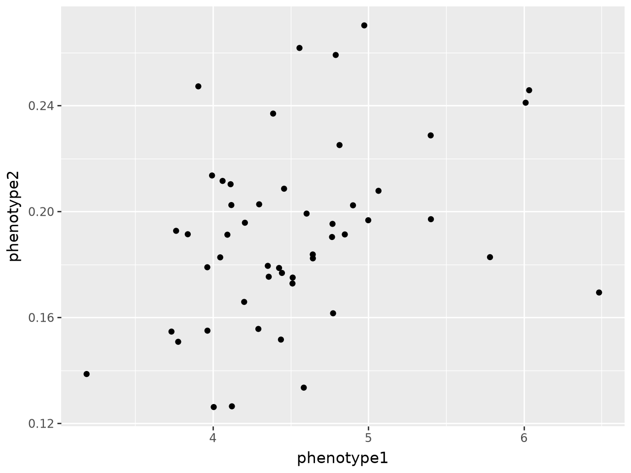
Here’s the joint distribution of trait values. The first is positive (since it’s multiplicative) and the second between 0 and 1 (since it’s logistic).
df >> p9.ggplot(p9.aes(x='phenotype1', y='phenotype2')) + p9.geom_point()
A “logistic” trait is just an additive trait that’s been put through the logistic transform, \(x \mapsto 1/(1 + \exp(-x))\). So we can use the code above to verify:
alive = pyslim.individuals_alive_at(ts, 0)
ind = ts.individual(alive[0])
ind_pheno = additive_genetic_value(ts, mut_metadata, ind) + additive_offset(ts_metadata, ind)
ind_pheno[1] = 1/(1 + np.exp(-ind_pheno[1]))
print(f"Ours: {ind_pheno}")
print(f"SLiM: {np.array([x['phenotype'] for x in ind.metadata['per_trait']])}")
Ours: [5.80340458 0.20239797]
SLiM: [4.11887898 0.20239797]
The second phenotype matches, since that’s the logistic trait. The first does not, as expected, since we’ve computed the phenotype as if it were additive, when in fact it’s multiplicative.
For the multiplicative trait, we need some new functions.
Following the pattern above,
and remembering that while the effects on an additive trait are
+(0, h*2*s, 2*s), for a multiplicative trait they are
*(1, 1+h*s, 1+s):
def multiplicative_effect(mut_metadata, a, b):
    # here a and b are *string* derived states
    num_traits = len(next(iter(mut_metadata.values()))['per_trait'])
    out = np.zeros((num_traits,))
    muts = Counter(a.split(",")) + Counter(b.split(","))
    for m in muts:
        if m != "":
            md = mut_metadata[int(m)]['per_trait']
            for j in range(num_traits):
                s = md[j]["effect_size"]
                if muts[m] == 1:
                    h = md[j]['dominance']
                    if np.isnan(h):
                        # "independent dominance occurs when (1+hs)(1+hs) equals 1+s,
                        # which occurs when h=(sqrt(1+s)−1)/s"
                        h = (np.sqrt(1 + s) - 1) / s if s != 0 else 0
                    out[j] *= (1 + h * s)
                else:
                    assert  muts[m] == 2
                    out[j] *= max(0, 1 + s)
    return out

# for instance, a homozygote for the first mutation:
mut = ts.mutation(0)
multiplicative_effect(mut_metadata, mut.derived_state, mut.derived_state)
array([0., 0.])
Genetic values:
def multiplicative_genetic_value(ts, mut_metadata, ind):
    out = np.ones((num_traits,))
    for v in ts.variants(samples=ind.nodes):
        x, y = [v.alleles[g] for g in v.genotypes]
        out *= multiplicative_effect(mut_metadata, x, y)
    return out

multiplicative_genetic_value(ts, mut_metadata, ts.individual(0))
array([0., 0.])
Offsets:
def multiplicative_offset(ts_metadata, ind):
    k = {
        pyslim.INDIVIDUAL_TYPE_HERMAPHRODITE : "baselineOffsetH",
        pyslim.INDIVIDUAL_TYPE_FEMALE : "baselineOffsetF",
        pyslim.INDIVIDUAL_TYPE_MALE : "baselineOffsetM",
    }[ind.metadata["sex"]]
    out = np.array([x[k] for x in ts_metadata['SLiM']['traits']])
    out *= [x['offset'] for x in ind.metadata['per_trait']]
    return out

multiplicative_offset(ts.metadata, ts.individual(0))
array([4.59723703, 0.07860051])
Let’s combine these into a function that works for this simulation.
This is not going to be very efficient (for many reasons),
but efficiency is not important here, since we’re just verifying that we understand
how the phenotype values SLiM computes relate to what’s in the tree sequence.
def phenotype(ind):
    out = multiplicative_offset(ts_metadata, ind)
    out[1] = additive_offset(ts_metadata, ind)[1]
    mult = multiplicative_genetic_value(ts, mut_metadata, ind)
    add = additive_genetic_value(ts, mut_metadata, ind)
    out[0] *= mult[0]
    out[1] += add[1]
    out[1] = 1 / (1 + np.exp(-out[1]))
    return out
Putting this together,
alive = pyslim.individuals_alive_at(ts, 0)
ind = ts.individual(alive[0])
print(f"Ours: {phenotype(ind)}")
print(f"SLiM: {np.array([x['phenotype'] for x in ind.metadata['per_trait']])}")
Ours: [0.         0.20239797]
SLiM: [4.11887898 0.20239797]
Happily, these again agree, up to floating point error.
More elegant code would pull the trait types out of top-level metadata and use additive or multiplicative effects accordingly, etcetera. Furthermore, if some chromosomes are not autosomes, we’d need to identify the ploidy of each individual, and use the hemizygous dominance coefficient when appropriate.
Technical details#
You’re better off using SLiM to calculate phenotypes than doing it yourself in python. There’s lots of corner cases, and phenotypes can even be modified by the SLiM script directly. But, there’s some situations where it’s important to know about those corner cases.
First: phenotypes are determined from the various contributions by
either a sum (“additive” or “logistic”) or a product (“multiplicative”).
Logistic traits are then transformed.
The contributions come from the global baselineOffsetX values
(which one depends on the sex of the individual),
from individual offsets, and from cumulative mutation effects.
The contribution of 0, 1, or 2 copies of a SLiM mutation to a diploid is either 0, 2hs, or 2s (additive) or 1, 1+hs, 1+s (multiplicative), where h is the dominance coefficient and s is the effect size. For a hemizygous individual, the contributions are the same (for 0 and 1 copies), but using the hemizygous dominance coefficient for h. For haploids, the contributions of 0 or 1 copy is either 0, 2s or 1, 1+s. For an individual without the chromosome at all, there is no effect (obviously).
Usually, that’s all we need to know.
However, there’s some more complications that affect the default trait
(i.e., the trait you get - called simT - if you don’t explicitly declare any traits),
or if you have set up a trait without baseline accumulation
and with mutations that convert to substitutions.
This can also be important to understand if you remove fixed mutations in python,
and then want to read the file back into SLiM:
to keep phenotypes the same, you have to include the effects of any removed mutations
that count towards the trait in the baselineOffsetX value.
Which mutations count?
Within SLiM, when a Mutation fixes, it might convert into a Substitution.
Whether this occurs is determined by
the mutation type’s convertToSubstitution property,
which is True by default in WF models and False by default in nonWF models.
Substitutions are no longer used by SLiM for calculating individual traits,
and so to retain the effects of fixed mutations,
sometimes scripts will set convertToSubstitution=F if it was not already set.
Another mechanism to retain these effects is the Trait property substitutionAccumulation,
which defaults to True.
If a trait has substitutionAccumulation=T, then the effects of any Substitutions
are accumulated in the “substitution offset”, and thus contribute to every individual’s
phenotype. The net effect of this is that the contributions of any mutations that fix
will be included in the phenotype values of all individuals
as long as convertToSubstitution=F for their mutation type,
or substitutionAccumulation=T for the trait, or both.
However, the tree sequence does not record whether a given mutation was converted to
a Substitution or not, and also does not record anything about mutation types,
including their convertToSubstitution property.
(This is because genome structure is set up before .trees files can be loaded.)
So, when we find a fixed mutation in the tree sequence, we don’t know a priori
if this is a Substitution or not.
If substitutionAccumulation=T for the trait
(information that is in the top-level metadata),
then it doesn’t matter, mutations will contribute either way.
The problematic combination: substitutionAccumulation=F and convertToSubstitution=T
is in most cases biologically undesireable, and only enabled for the default trait
for historical reasons.
In any case, the potentially missing information is in the script: are these mutation types
converting to substitutions or not?
Finally, a note on the substitutionOffsetX properties (where X is M, F, or H).
This is where SLiM stores the effect of any substitutions on the traits of
males, females, and heterozygotes, respectively.
These are distinct because of the differing effects of fixed mutations on individuals
when some individuals have different numbers of copies of a chromosome than other individuals.