Overview

A tree sequence is a way of storing both the full genetic history and the genotypes of a bunch of genomes. See the tskit documentation for more description of the tree sequence and underlying data structure, and definitions of the important terms. Each (haploid) genome is associated with a node, and the “focal” nodes are called sample nodes or simply samples. Many operations on tree sequences act on the sample nodes by default (see the tskit data model for more on this topic), and the tree sequence always describes the genealogy of the entire genome of all the samples, at at least over the simulated time period. (Other nodes in the tree sequence represent ancestral genomes about which we might have only partial information). SLiM simulates diploid organisms, so each individual usually has two nodes; many operations you might want to do involve first finding the individuals you want, and then looking at their nodes.

What does SLiM record in the tree sequence?

Suppose we’ve run a very small simulation with SLiM. The genetic relationships between the various diploid individuals who were alive over the course of the simulation might look something like the picture on the left below. Note that individuals (circles) are diploid, so that each contains two chromosomes or nodes (shaded rectangles), and that relationships are between the nodes, not the individuals.

At the end of the simulation we are typically only interested in the genetic relationships between the nodes in those individuals which are still alive; other parts of the genealogy are irrelevant. To save having to store this unnecessary genealogical information, SLiM simplifies the tree sequence as it goes along, retaining only certain parts of the genetic genealogy. When the tree sequence is output, the result then looks something like the situation in the figure below, in which many of the nodes and individuals have been removed.

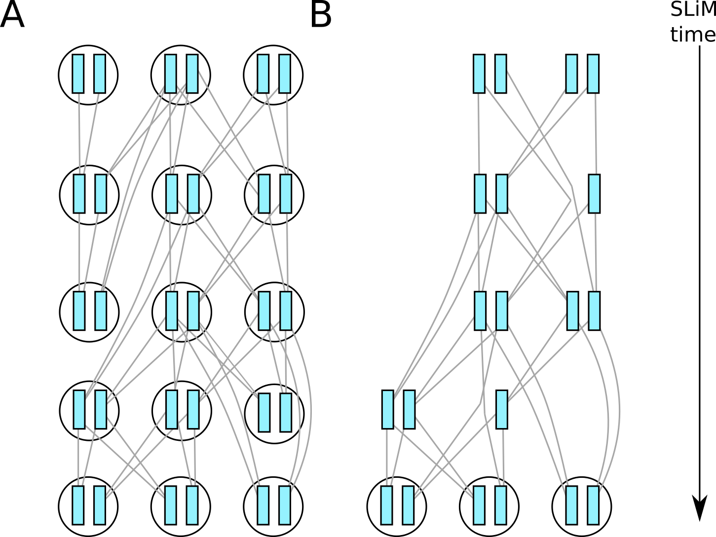
Fig. 1 A conceptual diagram of (A) relationships between chromosomes of diploid individuals in a SLiM simulation, and (B) which information is returned in the tree sequence.

Who and what is in the tree sequence?

OK, who and what exactly is left in the tree sequence after the unnecessary information has been removed? Figure 2 depicts the terminology.

Fig. 2 The diagram in figure 1, with labels.

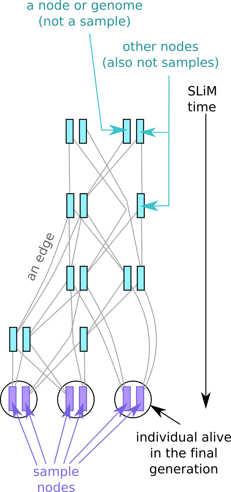
In the recorded tree sequence the individuals who are alive at the end of the simulation have their nodes marked as samples, and so we have their full genetic ancestry. The sample nodes, and the individuals containing them, are always present in the tree sequence.

In contrast to the individuals containing sample nodes, you can see that all the other circles, representing historical (i.e., dead) individuals, have vanished, although sometimes their nodes remain. By default, only individuals with sample nodes are recorded in the tree sequence; that means the other, remaining, nodes lose any information about which individuals they were in (the tutorial explains ways to retain this information.

As well as the historical individuals, many historical nodes have been removed too, along with with their genealogical relationships (i.e. the lines, which in tree-sequence-speak are known as “edges”). The deleted nodes are simply those that are not needed to reconstruct the relationships between the sample nodes. For example, we remove nodes leading to a dead end (e.g. in individuals who had no offspring). Similarly, as time goes on, recombination events in conjunction with genetic drift can gradually reduce the genetic contribution of parts of older genomes to the current generation. The generated tree sequence therefore need not contain historical nodes whose genetic contribution to the samples has been whittled down to zero. Finally, to reconstruct relationships between samples, strictly we only need to keep a node if it represents the genetic most recent common ancestor (MRCA) of at least two samples. So by default, we also remove historical nodes that are only “on the line to” a sample, but do not represent a branching point (i.e. coalescent event) on the tree.

What else can I find out from the tree sequence?

Enough information is stored in the tree sequence to completely reconstruct the state of the SLiM simulation (except for user-defined data, like a tag). Most of this is stored as metadata: see Metadata.

Vacant nodes: sex chromosomes and haploidy

Under the hood in SLiM, all individuals are diploid, and so for each individual there are two nodes, representing their two haplosomes (i.e., chromosome copies; see the SLiM manual). So, any individual that is not diploid for whichever chromosome the tree sequence represents will have in the tree sequence one or two nodes that don’t actually represent any genetic material. We call these vacant nodes. For instance, for a Y chromosome, each female individual will have two vacant nodes and males have one vacant node and one non-vacant node.

Vacant nodes have no ancestry information: no ancestors, no mutations, etcetera; just missing data. (You’ll see why they are in the tree sequence at all in the next section.)

Suppose that in the simulation of figure 1 we instead were simulating (only) a haploid, maternally-inherited chromosome (as for instance the mitochondria). If so, and the mitochondria are the left-hand nodes in each individual, then we’d get the tree sequence shown in figure 3.

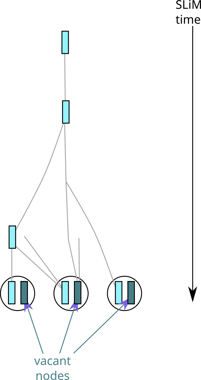
Fig. 3 What would be recorded in the simulation of figure 1, if we were simulating a haploid, maternally-inherited chromosome.

Multichromosome simulations

With SLiM v5, we have support for simulating multiple chromosomes simultaneously. In such a simulation, each chromosome is saved to a separate tree sequence in a “trees archive” (a directory of .trees files). Of course, the inheritance of those chromosomes all passed through the same set of ancestors, so it is natural that each of those tree sequences refer to the same set of nodes, individuals, and populations. So, the sets of nodes, individuals, and populations in all the tree sequences in a trees archive are identical. This is quite handy if you’re going to analyze data from more than one chromosome, but also creates some potential pitfalls.

First, there will probably be nodes in the tree sequence that are not represented in any of the trees. This is simply because these are nodes that are needed for other chromosomes: perhaps the node in question is not ancestral to any of the samples on this chromosome, but it is on other chromosomes. The presence of these nodes is harmless, however: it will not affect computation of statistics, they will not show up in tree traversals, they won’t appear in visualizations: for most purposes, they are invisible, because tskit’s data model is designed to pay attention to nodes that are ancestral to the samples. (See, for instance, on missing data.)

The rules for what is included in the tree sequence apply separately to each chromosome, then the resulting lists of nodes and individuals are combined. So, if a node is a coalescent node on one chromosome, and ancestral to the samples on another but not a coalescent node, then it would be present in both tree sequences but not used in the second one. For instance, all the nodes in figure 1 would be present as well in the tree sequence for figure 3, if both were from the same multichromosome simulation, and vice-versa.

Finally, this explains why vacant nodes must be included in the tree sequence: in the presence of autosomes, every diploid individual needs two nodes, but for an individual that has less than two copies of a given chromosome, some of those nodes will not represent an actual chromosome copy. Those are “vacant”, as described above.