Working with traits and phenotypes

Working with traits and phenotypes#

An individual’s phenotype for an trait in SLiM is the result of that individual’s genetic effects, and both global and individual-specific “offsets”. SLiM records in metadata both phenotype and offset, so we can use these (by subtraction, for an additive trait) to determine the genetic value. We can also compute genetic contributions directly, which can be helpful, for instance, to decompose genetic variance from different parts of the genome.

Let’s start off with this simulation, which has:

two additive traits,
with Gaussian selection on both,
started away from the optimum;
correlated mutational effects,
and also neutral mutations.

The recipe also saves the state of the population (by remembering everyone) every 1,000 generations. You may want to skip the details of the SLiM script on first reading.

initialize() {
	setSeed(123);
	initializeTreeSeq();
	defineConstant("START1", -5.0);
	defineConstant("START2", 5.0);
	defineConstant("OPT1", 20.0);
	defineConstant("OPT2", -20.0);
	initializeTrait("trait1", "additive", baselineOffset=START1, individualOffsetSD=1.0);
	initializeTrait("trait2", "additive", baselineOffset=START2, individualOffsetSD=1.0);
	
	initializeMutationType("m1", NAN, "f", 0.0);   // neutral
	initializeMutationType("m2", NAN, "f", 0.0);   // QTLs
	m2.color = "red";
	m2.logMutationData(enable=T, effectSize=T);
	m2.convertToSubstitution = F; // necessary to disentagle from baseline offset
	
	// g1 is a neutral region, g2 is a QTL
	initializeGenomicElementType("g1", m1, 1.0);
	initializeGenomicElementType("g2", c(m1,m2), c(1.0, 0.1));
	
	// chromosome of length 100 kb with two QTL regions
	initializeGenomicElement(g1, 0, 39999);
	initializeGenomicElement(g2, 40000, 49999);
	initializeGenomicElement(g1, 50000, 79999);
	initializeGenomicElement(g2, 80000, 89999);
	initializeGenomicElement(g1, 90000, 99999);
	initializeRecombinationRate(1e-8);
	initializeMutationRate(1e-7);
	
	// QTL-related constants used below
	defineConstant("QTL_mu", c(0.0, 0.0));
	defineConstant("QTL_cov", 0.25);
	defineConstant("QTL_sigma", matrix(c(1,QTL_cov,QTL_cov,1), nrow=2));
	}

1 late() {
	sim.addSubpop("p1", 500);
}

mutation(m2) {
	// draw mutational effects for the new m2 mutation
	effects = rmvnorm(1, QTL_mu, QTL_sigma);
	mut.setEffectSizeForTrait(NULL, effects);
	return T;
}

late() {
	sim.demandPhenotype(NULL, NULL);
	
	inds = sim.subpopulations.individuals;
	effects1 = 1.0 + dnorm(inds.trait1, OPT1, 15.0) * 10.0;
	effects2 = 1.0 + dnorm(inds.trait2, OPT2, 15.0) * 10.0;
	inds.fitnessScaling = effects1 * effects2;
}

1:1000000 late() {
	if (sim.cycle % 5000 == 0) {
		inds = p1.individuals;
		sim.treeSeqRememberIndividuals(inds);
		// keep running until we get close to both optima
		if ((abs(mean(inds.trait1) - OPT1) <= 1.0) & (abs(mean(inds.trait2) - OPT2) <= 1.0)) {
	   	sim.treeSeqOutput("phenotypes.trees", metadata=Dictionary("all_mutations", m2.loggedData("values")));
			sim.simulationFinished();
		}
	}
}

Trait distributions#

First, let’s load the result of the simulation and look at trait distributions in each of the saved time points.

ts = tskit.load("phenotypes.trees")
ts_metadata = ts.metadata
mut_metadata = pyslim.mutation_metadata(ts)

Here’s information about the traits:

ts_metadata['SLiM']['traits']

[{'baselineAccumulation': True,
  'baselineOffsetFromSubstitutions': 0.0,
  'baselineOffsetFromUser': -5.0,
  'directFitnessEffect': False,
  'index': 0,
  'individualOffsetMean': 0.0,
  'individualOffsetSD': 1.0,
  'name': 'trait1',
  'type': 'additive'},
 {'baselineAccumulation': True,
  'baselineOffsetFromSubstitutions': 0.0,
  'baselineOffsetFromUser': 5.0,
  'directFitnessEffect': False,
  'index': 1,
  'individualOffsetMean': 0.0,
  'individualOffsetSD': 1.0,
  'name': 'trait2',
  'type': 'additive'}]

Here’s the information we have about a given individual:

ts.individual(0)

Individual(id=0, flags=196608, location=array([0., 0., 0.]), parents=array([-1, -1], dtype=int32), nodes=array([6364, 6365], dtype=int32), metadata={'pedigree_id': 9999500, 'pedigree_p1': 9999327, 'pedigree_p2': 9999353, 'tag': -9223372036854775808, 'tagF': -1.7976931348623157e+308, 'age': -1, 'subpopulation': 1, 'sex': -1, 'tagL0_set': False, 'tagL0': False, 'tagL1_set': False, 'tagL1': False, 'tagL2_set': False, 'tagL2': False, 'tagL3_set': False, 'tagL3': False, 'tagL4_set': False, 'tagL4': False, 'per_trait': [{'phenotype': 21.577773274021574, 'offset': 1.7817394147686432}, {'phenotype': -19.403159486091294, 'offset': 0.5235182177661287}]})

In particular, phenotype and offset values:

ts.individual(0).metadata['per_trait']

[{'phenotype': 21.577773274021574, 'offset': 1.7817394147686432},
 {'phenotype': -19.403159486091294, 'offset': 0.5235182177661287}]

Next, let’s find the birth time of each individual, and see which times we have information for (this is simple because it’s a WF simulation):

ind_times = ts.nodes_time[ts.individuals_nodes[:,0]]

from collections import Counter
Counter([int(t) for t in ind_times])

Counter({0: 500, 15000: 500, 10000: 500, 5000: 500})

We can use the helpful metadata_vector method of table collections to quickly pull out the phenotype and offset vectors:

ind_phenotypes = np.column_stack([
    ts.tables.individuals.metadata_vector(["per_trait", j, "phenotype"])
    for j in (0, 1)
])
ind_offsets = np.column_stack([
    ts.tables.individuals.metadata_vector(["per_trait", j, "offset"])
    for j in (0, 1)
])

To prepare to make the plots (using plotnine) we’ll put everything in a data frame:

df = pd.DataFrame({
    'pedigree_id' : ts.tables.individuals.metadata_vector("pedigree_id"),
    'time' : ind_times,
    "phenotype1" : ind_phenotypes[:,0],
    "offset1" : ind_offsets[:,0],
    "phenotype2" : ind_phenotypes[:,1],
    "offset2" : ind_offsets[:,1],
})

As noted before, we can get the genetic contributions by subtracting the individual-level offsets:

df['genetic_value1'] = df['phenotype1'] - df['offset1']
df['genetic_value2'] = df['phenotype2'] - df['offset2']

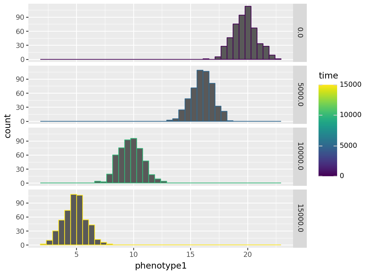
Now, here’s phenotype distributions across these time slices

( df >> 
    p9.ggplot(p9.aes(x='phenotype1', color="time"))
    + p9.geom_histogram(bins=40) + p9.facet_grid("time ~")
)

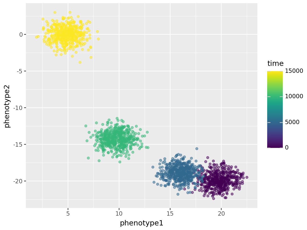
_images/1306205e958e32e5852cc2aac1a2911dc6f0409f7af4f1254b8b8e79b67847e3.png

Here’s how the population moved through 2d phenotype space:

(
    df >> p9.ggplot(p9.aes(x="phenotype1", y="phenotype2", color="time")) 
    + p9.geom_point(alpha=0.5)
)

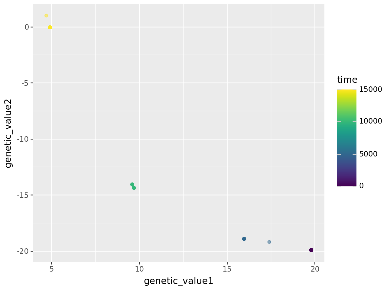
_images/0cbb5231c913d8251c80c8dfd6a47929981d9791e87a6a3cb24444d970b69459.png

That’s the phenotypes; it turns out that most of that spread is actually “offset”, i.e., what’s usually called “environmental” noise:

(
    df >> p9.ggplot(p9.aes(x="genetic_value1", y="genetic_value2", color="time")) 
    + p9.geom_point(alpha=0.5)
)

_images/eb0a53792aa35c38cfa3d1624b6ae8116e49b9ffdb89637aab9470f8ead69651.png

Mutation effects#

Now let’s see how to use mutation information to calculate genetic values directly. To do this, let’s take a simpler example. This just has two additive traits, and mutations have independent effects on each trait. There are two mutation types; the first is underdominant and the second is additive (using the special NAN value for $h$ to indicate independent dominance).

initialize() {
	setSeed(123);
	initializeTreeSeq(timeUnit="generations");
	initializeTrait("weight", "additive", baselineOffset=5.0, individualOffsetSD=0.2);
	initializeTrait("wing", "additive", baselineOffset=-1.0, individualOffsetSD=0.1);
	
	initializeMutationType("m1", 0.2, "n", 0.0, 0.01); 
	initializeMutationType("m2", NAN, "n", 0.0, 0.01); 
	
	initializeGenomicElementType("g1", c(m1,m2), c(0.5,0.5));
	
	initializeGenomicElement(g1, 0, 9999999);
	initializeRecombinationRate(1e-8);
	initializeMutationRate(1e-7);
}

1 late() {
	sim.addSubpop("p1", 50);
}

1000 late() {
	sim.demandPhenotype(NULL, NULL);
	sim.treeSeqOutput("phenotypes2.trees");
}

ts = tskit.load("phenotypes2.trees")
ts_metadata = ts.metadata
mut_metadata = pyslim.mutation_metadata(ts)

For example, here’s the first mutation:

mut = ts.mutation(0)
mut

Mutation(id=0, site=0, node=116, derived_state='98288', parent=-1, metadata={'derived_states': [98288]}, time=16.0, edge=261, inherited_state='')

We can see which SLiM mutation(s) this mutation represents by looking at the mutation’s “derived state”, and pulling the information out of the mutation metadata:

mut_metadata[mut.metadata["derived_states"][0]]

{'mutation_id': 98288,
 'mutation_type': 2,
 'subpopulation': 1,
 'slim_time': 984,
 'nucleotide': -1,
 'padding': None,
 'per_trait': [{'effect_size': -0.008490736596286297,
   'dominance': nan,
   'hemizygous_dominance': 1.0},
  {'effect_size': -4.386622822494246e-05,
   'dominance': nan,
   'hemizygous_dominance': 1.0}]}

So, we can use the effect_size and dominance to calculate genetic effects (we won’t need hemizygous dominance). Here is a function that calculates the effect of a pair of alleles. The function uses the derived_state property (a string) rather than the metadata property because that’s what’s returned by tskit.TreeSequence.variants(), which we’d like to use next.

from collections import Counter

def additive_effect(mut_metadata, a, b, num_traits=2):
    # here a and b are *string* derived states
    # note this works for additive traits:
    # multiplicative ones are "* (1 + hs)" instead of "+ 2hs"
    out = np.zeros((num_traits,))
    muts = Counter(a.split(",")) + Counter(b.split(","))
    for m in muts:
        if m != "":
            md = mut_metadata[int(m)]['per_trait']
            if muts[m] == 1:
                for j in range(num_traits):
                    h = md[j]['dominance']
                    if np.isnan(h):
                        h = 1/2
                    out[j] += 2 * md[j]['effect_size'] * h
            if muts[m] == 2:
                for j in range(num_traits):
                    out[j] += 2 * md[j]['effect_size']
    return out

# for instance, a homozygote for that mutation:
additive_effect(mut_metadata, mut.derived_state, mut.derived_state)

array([-1.69814732e-02, -8.77324564e-05])

Using this and tskit.TreeSequence.variants(), we can compute genetic values for an individual:

def additive_genetic_value(ts, mut_metadata, ind, num_traits=2):
    out = np.zeros((num_traits,))
    for v in ts.variants(samples=ind.nodes):
        x, y = [v.alleles[g] for g in v.genotypes]
        out += additive_effect(mut_metadata, x, y)
    return out

additive_genetic_value(ts, mut_metadata, ts.individual(0))

array([-0.11604283, -0.29277332])

The final component is offsets. To match SLiM we need to add in both the individual’s offset (which is stored in their metadata) and the global (“baseline”) offset. Within SLiM, the baselineOffset property is a sum of the value provided by the user on initialization of the trait, and the accumulated value of any substitutions (if various options do not modify this behavior; see the SLiM manual). Since the tree sequence does not distinguish substitutions from other mutations, SLiM stores these two components separately, as baselineOffsetFromUser and baselineOffsetFromSubstitutions. So, we just need to add in baselineOffsetFromUser.

def additive_offset(ts_metadata, ind):
    out = np.array([x['baselineOffsetFromUser'] for x in ts_metadata['SLiM']['traits']])
    out += [x['offset'] for x in ind.metadata['per_trait']]
    return out

additive_offset(ts.metadata, ts.individual(0))

array([ 4.83203513, -1.07860051])

Now we can compute phenotypes, and check they match what SLiM produced.

alive = pyslim.individuals_alive_at(ts, 0)
ind = ts.individual(alive[0])
print(f"Ours: {additive_genetic_value(ts, mut_metadata, ind) + additive_offset(ts_metadata, ind)}")
print(f"SLiM: {np.array([x['phenotype'] for x in ind.metadata['per_trait']])}")

Ours: [ 4.7159923  -1.37137383]
SLiM: [ 4.7159923  -1.37137383]

That looks good! To compare we need to account for floating-point error (actually the numbers stored by SLiM and computed by us may differ by $10^{-10}$).

for ind in ts.individuals():
    our_pheno = additive_genetic_value(ts, mut_metadata, ind) + additive_offset(ts_metadata, ind)
    slim_pheno = np.array([x['phenotype'] for x in ind.metadata['per_trait']])
    assert np.allclose(our_pheno, slim_pheno)

Multiplicative and logistic traits#

To see how multiplicative and logistic traits work, we’ll change the first trait to be multiplicative and the second logistic:

initialize() {
	setSeed(123);
	initializeTreeSeq(timeUnit="generations");
	initializeTrait("mult", "multiplicative", baselineOffset=5.0, individualOffsetSD=0.1);
	initializeTrait("logistic", "logistic", baselineOffset=-1.0, individualOffsetSD=0.1);
	
	initializeMutationType("m1", 0.2, "n", 0.0, 0.01); 
	initializeMutationType("m2", NAN, "n", 0.0, 0.01); 
	
	initializeGenomicElementType("g1", c(m1,m2), c(0.5,0.5));
	
	initializeGenomicElement(g1, 0, 9999999);
	initializeRecombinationRate(1e-8);
	initializeMutationRate(1e-7);
}

1 late() {
	sim.addSubpop("p1", 50);
}

1000 late() {
	sim.demandPhenotype(NULL, NULL);
	sim.treeSeqOutput("phenotypes3.trees");
}

This produces

ts = tskit.load("phenotypes3.trees")
ts_metadata = ts.metadata
mut_metadata = pyslim.mutation_metadata(ts)
ts

Tree Sequence
Trees	141
Sequence Length	10 000 000
Time Units	generations
Sample Nodes	100
Total Size	309.2 KiB
Metadata	dict SLiM: dict chromosomes: list dict id: 1 index: 0 name: A symbol: A type: A cycle: 1000 file_version: 1.0 model_type: WF name: sim nucleotide_based: False separate_sexes: False spatial_dimensionality: spatial_periodicity: stage: late this_chromosome: dict id: 1 index: 0 name: A symbol: A type: A tick: 1000 traits: list dict baselineAccumulation: True baselineOffsetFromSubstitutions: 0.8944892219804647 baselineOffsetFromUser: 5.0 directFitnessEffect: False index: 0 individualOffsetMean: 0.0 individualOffsetSD: 0.1 name: mult type: multiplicative dict baselineAccumulation: True baselineOffsetFromSubstitutions: -0.21228318789871992 baselineOffsetFromUser: -1.0 directFitnessEffect: False index: 1 individualOffsetMean: 0.0 individualOffsetSD: 0.1 name: logistic type: logistic SLiM_mutation_list: list dict mutation_id: 15 mutation_type: 1 subpopulation: 1 slim_time: 2 nucleotide: -1 padding: None per_trait: list dict effect_size: -0.026010943576693535 dominance: 0.20000000298023224 hemizygous_dominance: 1.0 dict effect_size: 0.003134363330900669 dominance: 0.20000000298023224 hemizygous_dominance: 1.0 dict mutation_id: 1576 mutation_type: 2 subpopulation: 1 slim_time: 17 nucleotide: -1 padding: None per_trait: list dict effect_size: 0.0020196049008518457 dominance: nan hemizygous_dominance: 1.0 dict effect_size: 0.009735784493386745 dominance: nan hemizygous_dominance: 1.0 dict mutation_id: 1987 mutation_type: 1 subpopulation: 1 slim_time: 21 nucleotide: -1 padding: None per_trait: list dict effect_size: 0.01020310539752245 dominance: 0.20000000298023224 hemizygous_dominance: 1.0 dict effect_size: 0.0009580525802448392 dominance: 0.20000000298023224 hemizygous_dominance: 1.0 dict mutation_id: 837 mutation_type: 2 subpopulation: 1 slim_time: 10 nucleotide: -1 padding: None per_trait: list dict effect_size: -0.009154281578958035 dominance: nan hemizygous_dominance: 1.0 dict effect_size: -0.00371098006144166 dominance: nan hemizygous_dominance: 1.0 dict mutation_id: 3126 mutation_type: 2 subpopulation: 1 slim_time: 32 nucleotide: -1 padding: None per_trait: list dict effect_size: 0.0012267092242836952 dominance: nan hemizygous_dominance: 1.0 dict effect_size: -0.0011492078192532063 dominance: nan hemizygous_dominance: 1.0 dict mutation_id: 1703 mutation_type: 1 subpopulation: 1 slim_time: 18 nucleotide: -1 padding: None per_trait: list dict effect_size: -0.004852541256695986 dominance: 0.20000000298023224 hemizygous_dominance: 1.0 dict effect_size: 0.002290119417011738 dominance: 0.20000000298023224 hemizygous_dominance: 1.0 dict mutation_id: 2796 mutation_type: 2 subpopulation: 1 slim_time: 29 nucleotide: -1 padding: None per_trait: list dict effect_size: -0.002255016239359975 dominance: nan hemizygous_dominance: 1.0 dict effect_size: -0.0017606235342100263 dominance: nan hemizygous_dominance: 1.0 dict mutation_id: 1988 mutation_type: 2 subpopulation: 1 slim_time: 21 nucleotide: -1 padding: None per_trait: list dict effect_size: 0.02024916745722294 dominance: nan hemizygous_dominance: 1.0 dict effect_size: 0.005838510114699602 dominance: nan hemizygous_dominance: 1.0 dict mutation_id: 3400 mutation_type: 2 subpopulation: 1 slim_time: 35 nucleotide: -1 padding: None per_trait: list dict effect_size: 0.01987594924867153 dominance: nan hemizygous_dominance: 1.0 dict effect_size: 0.015985509380698204 dominance: nan hemizygous_dominance: 1.0 dict mutation_id: 1313 mutation_type: 2 subpopulation: 1 slim_time: 15 nucleotide: -1 padding: None per_trait: list dict effect_size: -0.00017658188880886883 dominance: nan hemizygous_dominance: 1.0 dict effect_size: -0.015020333230495453 dominance: nan hemizygous_dominance: 1.0 dict mutation_id: 1190 mutation_type: 2 subpopulation: 1 slim_time: 13 nucleotide: -1 padding: None per_trait: list dict effect_size: -0.014724056236445904 dominance: nan hemizygous_dominance: 1.0 dict effect_size: 0.002498218324035406 dominance: nan hemizygous_dominance: 1.0 dict mutation_id: 2064 mutation_type: 2 subpopulation: 1 slim_time: 22 nucleotide: -1 padding: None per_trait: list dict effect_size: 0.007496724370867014 dominance: nan hemizygous_dominance: 1.0 dict effect_size: -0.0011577224358916283 dominance: nan hemizygous_dominance: 1.0 dict mutation_id: 3854 mutation_type: 1 subpopulation: 1 slim_time: 40 nucleotide: -1 padding: None per_trait: list dict effect_size: 0.010805635713040829 dominance: 0.20000000298023224 hemizygous_dominance: 1.0 dict effect_size: 0.003640131326392293 dominance: 0.20000000298023224 hemizygous_dominance: 1.0 dict mutation_id: 869 mutation_type: 1 subpopulation: 1 slim_time: 10 nucleotide: -1 padding: None per_trait: list dict effect_size: -0.017547879368066788 dominance: 0.20000000298023224 hemizygous_dominance: 1.0 dict effect_size: 0.0006886860937811434 dominance: 0.20000000298023224 hemizygous_dominance: 1.0 dict mutation_id: 1175 mutation_type: 2 subpopulation: 1 slim_time: 13 nucleotide: -1 padding: None per_trait: list dict effect_size: -0.013079150579869747 dominance: nan hemizygous_dominance: 1.0 dict effect_size: -0.005980576388537884 dominance: nan hemizygous_dominance: 1.0 dict mutation_id: 232 mutation_type: 1 subpopulation: 1 slim_time: 4 nucleotide: -1 padding: None per_trait: list dict effect_size: 0.0033567564096301794 dominance: 0.20000000298023224 hemizygous_dominance: 1.0 dict effect_size: 0.01929246261715889 dominance: 0.20000000298023224 hemizygous_dominance: 1.0 dict mutation_id: 321 mutation_type: 2 subpopulation: 1 slim_time: 5 nucleotide: -1 padding: None per_trait: list dict effect_size: -0.002490913262590766 dominance: nan hemizygous_dominance: 1.0 dict effect_size: -0.011669306084513664 dominance: nan hemizygous_dominance: 1.0 dict mutation_id: 2692 mutation_type: 1 subpopulation: 1 slim_time: 28 nucleotide: -1 padding: None per_trait: list dict effect_size: 0.018162688240408897 dominance: 0.20000000298023224 hemizygous_dominance: 1.0 dict effect_size: 0.0029179221019148827 dominance: 0.20000000298023224 hemizygous_dominance: 1.0 dict mutation_id: 4078 mutation_type: 1 subpopulation: 1 slim_time: 42 nucleotide: -1 padding: None per_trait: list dict effect_size: 0.017629289999604225 dominance: 0.20000000298023224 hemizygous_dominance: 1.0 dict effect_size: -0.007538866717368364 dominance: 0.20000000298023224 hemizygous_dominance: 1.0 dict mutation_id: 2703 mutation_type: 1 subpopulation: 1 slim_time: 28 nucleotide: -1 padding: None per_trait: list dict effect_size: -0.010814151726663113 dominance: 0.20000000298023224 hemizygous_dominance: 1.0 dict effect_size: 0.0027240614872425795 dominance: 0.20000000298023224 hemizygous_dominance: 1.0 dict mutation_id: 852 mutation_type: 1 subpopulation: 1 slim_time: 10 nucleotide: -1 padding: None per_trait: list dict effect_size: 0.00402882369235158 dominance: 0.20000000298023224 hemizygous_dominance: 1.0 dict effect_size: 0.003662815084680915 dominance: 0.20000000298023224 hemizygous_dominance: 1.0 dict mutation_id: 3384 mutation_type: 1 subpopulation: 1 slim_time: 35 nucleotide: -1 padding: None per_trait: list dict effect_size: -0.0024172388948500156 dominance: 0.20000000298023224 hemizygous_dominance: 1.0 dict effect_size: -0.0008700435282662511 dominance: 0.20000000298023224 hemizygous_dominance: 1.0 dict mutation_id: 4144 mutation_type: 2 subpopulation: 1 slim_time: 43 nucleotide: -1 padding: None per_trait: list dict effect_size: -0.01489799004048109 dominance: nan hemizygous_dominance: 1.0 dict effect_size: -4.0450362575938925e-05 dominance: nan hemizygous_dominance: 1.0 dict mutation_id: 3873 mutation_type: 2 subpopulation: 1 slim_time: 40 nucleotide: -1 padding: None per_trait: list dict effect_size: -0.010952734388411045 dominance: nan hemizygous_dominance: 1.0 dict effect_size: -0.0005257998127490282 dominance: nan hemizygous_dominance: 1.0 dict mutation_id: 2427 mutation_type: 2 subpopulation: 1 slim_time: 25 nucleotide: -1 padding: None per_trait: list dict effect_size: 0.004659339319914579 dominance: nan hemizygous_dominance: 1.0 dict effect_size: 0.01215437613427639 dominance: nan hemizygous_dominance: 1.0 dict mutation_id: 2129 mutation_type: 2 subpopulation: 1 slim_time: 22 nucleotide: -1 padding: None per_trait: list dict effect_size: 0.005004825536161661 dominance: nan hemizygous_dominance: 1.0 dict effect_size: -0.003335549496114254 dominance: nan hemizygous_dominance: 1.0 dict mutation_id: 5279 mutation_type: 2 subpopulation: 1 slim_time: 54 nucleotide: -1 padding: None per_trait: list dict effect_size: -0.012746073305606842 dominance: nan hemizygous_dominance: 1.0 dict effect_size: 0.004763415548950434 dominance: nan hemizygous_dominance: 1.0 dict mutation_id: 4016 mutation_type: 1 subpopulation: 1 slim_time: 41 nucleotide: -1 padding: None per_trait: list dict effect_size: 0.008188897743821144 dominance: 0.20000000298023224 hemizygous_dominance: 1.0 dict effect_size: 0.005705110263079405 dominance: 0.20000000298023224 hemizygous_dominance: 1.0 dict mutation_id: 853 mutation_type: 2 subpopulation: 1 slim_time: 10 nucleotide: -1 padding: None per_trait: list dict effect_size: 0.0007417929591611028 dominance: nan hemizygous_dominance: 1.0 dict effect_size: -0.007455283775925636 dominance: nan hemizygous_dominance: 1.0 dict mutation_id: 5561 mutation_type: 2 subpopulation: 1 slim_time: 57 nucleotide: -1 padding: None per_trait: list dict effect_size: 0.0032693573739379644 dominance: nan hemizygous_dominance: 1.0 dict effect_size: -0.014267022721469402 dominance: nan hemizygous_dominance: 1.0 ... and 2055 more

Table	Rows	Size	Has Metadata
Edges	639	20.0 KiB
Individuals	50	11.3 KiB	✅
Migrations	0	8 Bytes
Mutations	2 085	100.3 KiB	✅
Nodes	285	11.9 KiB	✅
Populations	2	2.3 KiB	✅
Provenances	1	4.0 KiB
Sites	2 084	48.9 KiB

Provenance Timestamp	Software Name	Version	Command	Full record
01 September, 2026 at 03:32:34 PM	SLiM	5.2	['slim', '-s', '23', 'phenotypes3.slim']	Details dict environment: dict os: dict machine: x86_64 node: runnervmgx7h7 release: 6.17.0-1022-azure system: Linux version: #22-Ubuntu SMP Mon Jul 27 17:24:03 UTC 2026 metadata: dict individuals: dict flags: dict 16: dict description: the individual was alive at the time the file was written name: SLIM_TSK_INDIVIDUAL_ALIVE 17: dict description: the individual was requested by the user to be permanently remembered name: SLIM_TSK_INDIVIDUAL_REMEMBERED 18: dict description: the individual was requested by the user to be retained only if its nodes continue to exist in the t... name: SLIM_TSK_INDIVIDUAL_RETAINED 19: dict description: the individual is a recent migrant between subpopulations name: SLIM_TSK_INDIVIDUAL_MIGRATED parameters: dict chromosomes: list dict id: 1 index: 0 name: A symbol: A type: A command: list slim -s 23 phenotypes3.slim model: initialize() { setSeed(123); initiali zeTreeSeq(timeUnit="generation s"); initializeTrait("mult", "... model_hash: ae381a780b14a6fc47e909cc06414c 13b784be444c2578704495f828ae17 f496 model_type: WF nucleotide_based: False seed: 23 separate_sexes: False spatial_dimensionality: spatial_periodicity: stage: late this_chromosome: dict id: 1 index: 0 name: A symbol: A type: A traits: list dict baselineAccumulation: True baselineOffsetFromSubstitutions: 0.8944892219804647 baselineOffsetFromUser: 5.0 directFitnessEffect: False index: 0 individualOffsetMean: 0.0 individualOffsetSD: 0.1 name: mult type: multiplicative dict baselineAccumulation: True baselineOffsetFromSubstitutions: -0.21228318789871992 baselineOffsetFromUser: -1.0 directFitnessEffect: False index: 1 individualOffsetMean: 0.0 individualOffsetSD: 0.1 name: logistic type: logistic resources: dict elapsed_time: 0.163518946 max_memory: 18923520 sys_time: 0.021899 user_time: 0.143341 schema_version: 1.1.0 slim: dict cycle: 1000 file_version: 1.0 name: sim tick: 1000 software: dict name: SLiM version: 5.2

To cite this software, please consult the citation manual: https://tskit.dev/citation/

Just for the heck of it, we’ll load the information into a data frame row-wise instead of column-wise:

df = pd.DataFrame([
        (
         ts.node(ind.nodes[0]).time,
         ind.metadata['per_trait'][0]['phenotype'],
         ind.metadata['per_trait'][0]['offset'],
         ind.metadata['per_trait'][1]['phenotype'],
         ind.metadata['per_trait'][1]['offset'],
        )
        for ind in ts.individuals()
    ],
    columns=['time', "phenotype1", "offset1", "phenotype2", "offset2"],
)

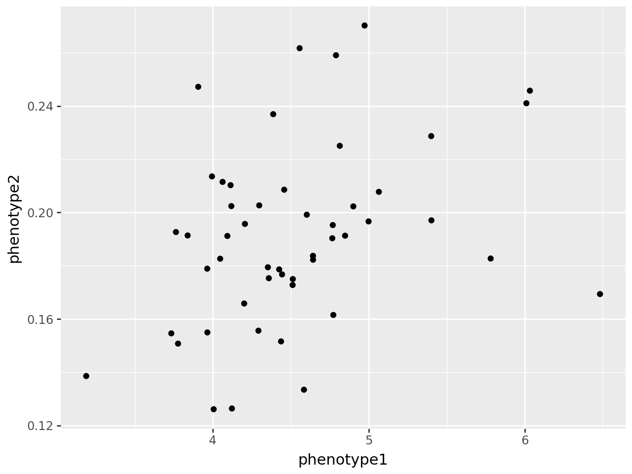
Here’s the joint distribution of trait values. The first is positive (since it’s multiplicative) and the second between 0 and 1 (since it’s logistic).

df >> p9.ggplot(p9.aes(x='phenotype1', y='phenotype2')) + p9.geom_point()

_images/bb4d27b483b3df8b786b361309e3def0693ff10a4d86f005abbf12aaf2e28e25.png

A “logistic” trait is just an additive trait that’s been put through the logistic transform, $x \mapsto 1/(1 + \exp(-x))$. So we can use the code above to verify:

alive = pyslim.individuals_alive_at(ts, 0)
ind = ts.individual(alive[0])
ind_pheno = additive_genetic_value(ts, mut_metadata, ind) + additive_offset(ts_metadata, ind)
ind_pheno[1] = 1/(1 + np.exp(-ind_pheno[1]))
print(f"Ours: {ind_pheno}")
print(f"SLiM: {np.array([x['phenotype'] for x in ind.metadata['per_trait']])}")

Ours: [5.80340458 0.20239797]
SLiM: [4.11887898 0.20239797]

For the multiplicative trait, we need some new functions. Following the pattern above:

def multiplicative_effect(mut_metadata, a, b, num_traits=2):
    # here a and b are *string* derived states
    out = np.ones((num_traits,))
    muts = Counter(a.split(",")) + Counter(b.split(","))
    for m in muts:
        if m != "":
            md = mut_metadata[int(m)]['per_trait']
            if muts[m] == 1:
                for j in range(num_traits):
                    h = md[j]['dominance']
                    if np.isnan(h):
                        h = 1/2
                    out[j] *= (1 + md[j]['effect_size'] * h)
            if muts[m] == 2:
                for j in range(num_traits):
                    out[j] *= (1 + md[j]['effect_size'])
    return out

# for instance, a homozygote for the first mutation:
mut = ts.mutation(0)
multiplicative_effect(mut_metadata, mut.derived_state, mut.derived_state)

array([0.99150926, 0.99995613])

Genetic values:

def multiplicative_genetic_value(ts, mut_metadata, ind, num_traits=2):
    out = np.ones((num_traits,))
    for v in ts.variants(samples=ind.nodes):
        x, y = [v.alleles[g] for g in v.genotypes]
        out *= multiplicative_effect(mut_metadata, x, y)
    return out

multiplicative_genetic_value(ts, mut_metadata, ts.individual(0))

array([0.89633798, 0.82445491])

Offsets:

def multiplicative_offset(ts_metadata, ind):
    out = np.array([x['baselineOffsetFromUser'] for x in ts_metadata['SLiM']['traits']])
    out *= [x['offset'] for x in ind.metadata['per_trait']]
    return out

multiplicative_offset(ts.metadata, ts.individual(0))

array([4.59723703, 0.07860051])

Let’s combine these into a function that works for this simulation. This is not going to be very efficient (for many reasons), but efficiency is not important here, since we’re just verifying that we understand how the phenotype values SLiM computes relate to what’s in the tree sequence.

def phenotype(ind):
    out = multiplicative_offset(ts_metadata, ind)
    out[1] = additive_offset(ts_metadata, ind)[1]
    add = additive_genetic_value(ts, mut_metadata, ind)
    mult = multiplicative_genetic_value(ts, mut_metadata, ind)
    out[0] *= mult[0]
    out[1] += add[1]
    out[1] = 1 / (1 + np.exp(-out[1]))
    return out

phenotype(ts.individual(0))

array([4.12067815, 0.20239797])

Putting this together,

alive = pyslim.individuals_alive_at(ts, 0)
ind = ts.individual(alive[0])
print(f"Ours: {phenotype(ind)}")
print(f"SLiM: {np.array([x['phenotype'] for x in ind.metadata['per_trait']])}")

Ours: [4.12067815 0.20239797]
SLiM: [4.11887898 0.20239797]

More elegant code would pull the trait types out of top-level metadata and use additive or multiplicative effects accordingly, etcetera.

Working with traits and phenotypes

Contents

Working with traits and phenotypes#

Trait distributions#

Mutation effects#

Multiplicative and logistic traits#