TSKIT 1.0.0!

The 1.0.0 release of tskit tags the point at which backwards compatibility is guaranteed for users. From now on, unless unavoidable (e.g. bugfixes), there should be no breaking changes to the API. We have taken the opportunity to fix minor inconsistencies in the data model, and provide several new ways to access underlying data more efficiently.

Many improvements and new capabilities have also accumulated since the previous 0.6.0 release. As well as bugfixes, these include several additional convenience arrays, a basic implementation of PCA analysis that scales to thousands of genomes or more, and an optional wrapper to speed up Python-based tree sequence algorithms using Numba, allowing traversal both up and down the graph (ARG) representation of a tree sequence.

Breaking changes

See the changelog for a full list: below are the two major ones

• The ts.tables attribute now returns an ImmutableTableCollection, meaning that you can’t change the resulting tables (to edit them, use the ts.dump_tables() method instead, which has always been the recommended editing method).
• The ordering requirement for mutations that occur at the same site has been tightened up. This stricter order is required to create a tree sequence, and the tables.sort() function now enforces the correct order (this allows efficient calculation of a mutation’s previous (“inherited”) and new (“derived”) state, allowing access to a mutation.inherited_state property, see below).

New features

Convenience arrays

Thanks to Ben Jeffery, the following are now available

Arrays of variable-length strings (requires NumPy 2.0)

• ts.sites_ancestral_state
• ts.mutations_derived_state
• ts.mutations_inherited_state
• ts.mutations_inherited_state

Convenience arrays (matching previous arrays such as ts.individual_populations, ts.individual_times etc):

• ts.mutations_edge
• ts.individual_nodes
• ts.sample_nodes_by_ploidy

A quick demonstration (including the new inherited_state property)

>>> import msprime
>>> import numpy as np
>>> ts = msprime.sim_ancestry(4, sequence_length=5, random_seed=123)
>>> ts = msprime.sim_mutations(ts, rate=0.1, random_seed=123)
>>> np.set_printoptions(formatter={'float': '{:0.1f}'.format}) # for nicer lining up
>>> print("Mutation positions:       ", ts.sites_position[ts.mutations_site])
>>> pos = ts.sites_position  # Or equivalently ts.tables.sites.position, which is now efficient
>>> print("Mutation ancestral states:", ts.sites_ancestral_state[ts.mutations_site])
>>> print("Mutation inherited states:", ts.mutations_inherited_state)
>>> print("Two nodes for each diploid individual:\n", ts.individuals_nodes)

>>> ts.draw_svg(
        title="Demo of inherited states, individual nodes, and a legend",
        size=(600, 300),
        mutation_labels={m.id:f"{m.inherited_state}{int(pos[m.site])}{m.derived_state}" for m in ts.mutations()},
        style="".join(".leaf.i%d .sym {fill: %s}" % x for x in enumerate(['red', 'green', 'blue', 'magenta'])),
        preamble="".join([
            f'<g transform="translate(40, {30 + 18*i})" class="leaf i{i}">'  # an SVG group
            f'<rect width="6" height="6" class="sym" /><text x="10" y="7">Ind {i}</text></g>'  # Label
            for i in range(ts.num_individuals)
        ])
    )

Mutation positions:        [0.0 1.0 2.0 2.0 3.0]
Mutation ancestral states: ['G' 'G' 'C' 'C' 'G']
Mutation inherited states: ['G' 'G' 'C' 'A' 'G']
Two nodes for each diploid individual:
 [[0 1]
 [2 3]
 [4 5]
 [6 7]]

You can see that the mutations at position 2 go from C to A to C, so that the most recent mutation at that position, above node 6, inherits the state “A” (right hand branch), even though the ancestral state at that locus is “C”. The code above also illustrates new arguments to the .draw_svg() methods, specifically preamble which can be used to create legends, and title.

PCA

Thanks to work by Hanbin Lee, Peter Ralph and others, there is now a scalable implementation of branch-based principle components analysis, which also allows windowing along the genome and by time (also see the previous news item). Further improvements to the ts.pca method are also planned.

>>> from matplotlib import pyplot as plt
>>> popn_colours = np.array(['steelblue', 'coral', 'limegreen', 'gold'])
>>> ts = msprime.sim_ancestry(
        samples={i: 10 for i in range(len(popn_colours))},
        demography=msprime.Demography.island_model([1e4] * len(popn_colours), migration_rate=1e-5),
        random_seed=1234,
        sequence_length=1e6,
        recombination_rate=1e-9
    )
>>> # Call the PCA
>>> pca_output = ts.pca(2)
>>> 
>>> # Plot it (output as scatter plot shown below)
>>> plt.scatter(*pca_output.factors.T, c=popn_colours[ts.nodes_population[ts.samples()]])
>>> plt.legend(handles = [
        plt.Line2D([], [], marker='o', c='w', mfc=c, ms=8, label=f"Pop {i}") for i, c in enumerate(popn_colours)
    ]);

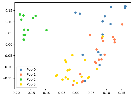
Try it out in the new interactive workbooks at http://tskit.dev/explore/.

Fast metadata access

For large tree sequences, accessing metadata can be a time consuming step. Now, if metadata uses the efficient struct codec, it is possible to access it as an efficient numpy array, e.g. via ts.individuals_metadata, ts.populations_metadata, etc. The new functionality is documented here. Below is a demo:

>>> import msprime
>>> import tskit
>>> # Make a tree sequence with some population metadata, 
>>> demog = msprime.Demography.island_model([1e4] * 4, migration_rate=1e-5)
>>> ts = msprime.sim_ancestry(samples={i: 10 for i in range(4)}, demography=demog)

>>> # Convert the metadata schema to a struct codec
>>> tables = ts.dump_tables()
>>> tables.populations.clear()
>>> schema = ts.tables.populations.metadata_schema.schema
>>> tables.populations.metadata_schema = tskit.MetadataSchema({
        "codec":"struct",
        "properties":{
            "description":{"binaryFormat":"10s","nullTerminated":True,"type":"string"},
            "name":{"binaryFormat":"10s","nullTerminated":True,"type":"string"}},
        "required":["name","description"],
        "type":"object",
    })
>>> for p in ts.populations():
        tables.populations.append(p)
>>> struct_ts = tables.tree_sequence()
>>> # Now we can get a "binary" numpy string array (more efficient for millions of entries)
>>> numpy_array = struct_ts.populations_metadata['name']
>>> assert numpy_array[0] == b'pop_0'

Although more restrictive than using json metadata, the resulting efficiency can be worth it for tables of millions of rows. For example, it enables fast analysis of our ARG of ~2.5 million SARS-CoV2 genomes, which you can explore in our interactive sc2ts notebook.

Numba integration

Work by Jerome Kelleher and Ben Jeffery makes it possible to speed up python-based tskit algorithms, sometimes by many orders of magnitude, using the Numba just-in-time (JIT) compiler.

This advanced tskit usage is primarily aimed at developers of new algorithms, hence Numba is only an optional tskit dependency. Its use is described in new documentation page, which also details how it can be used to traverse timewards through the tree sequence graph.

Other new features

The changelog describes a few more new features. Two in particular are:

• ts.concatenate() now exists, to convert multiple tree sequences along a genome into a single long tree sequence (also see ts.shift())
• Various improvements have been made to VCF exporting.