Usage#
We’ll first generate a few example “undated” tree sequences:
* Simulated `sim_ts` (20 genomes from a popn of 100 diploids, mut_rate=1e-06 /bp/gen)
* Inferred `inf_ts` using tsinfer (40 samples of human chr1:10000000-11000000)
Quickstart#
Given a known genetic genealogy in the form of a tree sequence, tsdate simply
re-estimates the node times based on the mutations on each edge. Usage is as
simple as calling the date() function with an
estimated per base pair per generation mutation rate.
import tsdate
# Running `tsdate` is usually a single function call, as follows:
mu_per_bp_per_generation = 1e-6
redated_ts = tsdate.date(sim_ts, mutation_rate=mu_per_bp_per_generation)
This simple example has no recombination, infinite sites mutation, a high mutation rate, and a known genealogy, so we would expect that the node times as estimated by tsdate from the mutations would be very close to the actual node times, as indeed they seem to be:
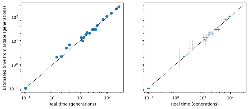
The left hand plot shows the redated tree sequence node times. The right hand plot is essentially identical but with 95% confidence intervals (technically, it shows the unconstrained posterior node times, with confidence intervals based on the gamma distribution fitted by the default tsdate method).
Note
By default time is assumed to be measured in “generations”, but this can be changed by
using the time_units parameter: see the Timescale adjustment section.
Inferred topologies#
A more typical use-case is where the genealogy has been inferred from DNA sequence data,
for example by tsinfer or
Relate. Below we will demonstrate with tsinfer
output based on DNA sequences generated by a more realistic simulation.
With real data, especially from tsinfer you may want to preprocess
the tree sequence before dating. This removes regions with no variable sites,
also simplifies to remove locally unary portions of nodes, and splits disjoint nodes
into separate datable nodes (see the
Preprocessing section for more details)
import tsdate
simplified_ts = tsdate.preprocess_ts(
    inf_ts,
    remove_telomeres=False  # Simulated example, so no flanking regions / telomeres exist
)
dated_ts = tsdate.date(simplified_ts, mutation_rate=model.mutation_rate)
print(
    f"Dated `inf_ts` (inferred from {inf_ts.num_sites} variants under the {model.id}",
    f"stdpopsim model, mutation rate = {model.mutation_rate} /bp/gen)"
)
Dated `inf_ts` (inferred from 3861 variants under the AmericanAdmixture_4B18 stdpopsim model, mutation rate = 2.36e-08 /bp/gen)
Note
In simulated data you may not have missing data regions, and you may be able to
pass erase_flanks=False to the preprocess_ts function.
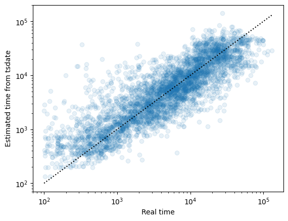
The inference in this case is much more noisy (as illustrated using the original and inferred times of the node under each mutation):
Note that if a bifurcating topology in the original genealogies has been collapsed
into a polytomy (multifurcation) in the inferred version, then the default node
times output by tsdate correspond to the time of the oldest bifurcating node.
If you wish to consider diversity or coalescence over time, you should therefore
consider explicitly setting the match_segregating_sites parameter to True
(see the Rescaling details section).
Results and posteriors#
The default output of tsdate is a new, dated tree sequence, created with node times set to the (constrained) posterior mean time for each node, and mutation times set halfway between the time of the node above and the time of the node below the mutation.
However, these tree-sequence time arrays do not capture all the information about the distribution of times. They do not contain information about the variance in the time estimates, and if necessary, mean times are constrained to create a valid tree sequence (i.e. if the mean time of a child node is older than the mean time of all of its parents, a small value, \(\epsilon\), is added to the parent time to ensure a valid tree sequence).
For this reason, there are two ways to get variances and unconstrained dates when running tsdate:
The nodes and mutations in the tree sequence will usually contain Metadata specifying mean time and its variance. These metadata values (currently saved as
mnandvr) are not constrained by the topology of the tree sequence, and should be used in preference e.g. tonodes_timeandmutations_timewhen evaluating the accuracy of tsdate.The
return_fitparameter can be used when callingtsdate.date(), which then returns both the dated tree sequence and a fit object. This object can then be queried for the unconstrained posterior distributions using e.g..node_posteriors()which can be read in to a pandas dataframe, as below:
import pandas as pd
redated_ts, fit = tsdate.date(
    sim_ts, mutation_rate=1e-6, return_fit=True)
posteriors_df = pd.DataFrame(fit.node_posteriors())  # mutation_posteriors() also available
posteriors_df.tail()  # Show the dataframe
| mean | variance | |
|---|---|---|
| 34 | 77.573465 | 26.359205 |
| 35 | 105.464187 | 30.020537 |
| 36 | 141.468529 | 52.913873 |
| 37 | 215.321172 | 56.009024 |
| 38 | 263.365664 | 69.361473 |
Timescale adjustment#
The default tsdate timescale is “generations”. Changing this can be as simple as
providing a time_units argument:
mu_per_bp_per_gen = 1e-8  # per generation
ts_generations = tsdate.date(ts, mutation_rate=mu_per_bp_per_gen)

mu_per_bp_per_year = 3.4e-10  # Human generation time ~ 29 years
ts_years = tsdate.date(ts, mutation_rate=mu_per_bp_per_year, time_units="years")
However, if you are specifying a node-specific prior, e.g. because you are using a
discrete-time method, you will also need to change the scale of the prior. In particular,
if you are setting the prior using the population_size argument, you will also need to
modify that by multiplying it by the generation time. For example:
Ne = 100  # Diploid population size
mu_per_bp_per_gen = 1e-8  # per generation
ts_generations = tsdate.inside_outside(ts, mutation_rate=mu_per_bp_per_gen, population_size=Ne)

# To infer dates in years, adjust both the rates and the population size:
generation_time = 29  # Years
mu_per_bp_per_year = mu_per_bp_per_gen / generation_time
ts_years = tsdate.inside_outside(
    ts,
    mutation_rate=mu_per_bp_per_year,
    population_size=Ne * generation_time,
    time_units="years"
)

# Check that the inferred node times are identical, just on different scales
assert np.allclose(ts_generations.nodes_time, ts_years.nodes_time / generation_time, 5)
Memory and run time#
Tsdate can be run on most modern computers. Using the default variational_gamma
method, large tree sequences of millions or
tens of millions of edges take tens of minutes and gigabytes of RAM (e.g. 10 GB / 50 mins
on a 2024-era Apple M2 laptop for a tree sequence of 65 million edges covering
81 megabases of 2.85 million samples of human chromosome 17 from
Anderson-Trocmé et al. [2023]).

Running the dating algorithm is linear in the number of edges in the tree sequence.
This makes tsdate usable even for vary large tree sequences (e.g. millions of samples).
For large instances, if you are running tsdate interactively, it can be useful to
specify the progress option to display a progress bar telling you how long
different stages of dating will take.
As the time taken to date a tree sequence using tsdate is only a fraction of that required to infer the initial tree sequence, the core tsdate algorithm has not been parallelised to allow running on many CPU cores.
CLI use#
Computationally-intensive uses of tsdate are likely to involve running the program non-interactively, e.g. as part of an automated pipeline. In this case, it may be useful to use the command-line interface. See Command line interface for more details.