Population size#
The rate of coalescence events over time is determined by demographics,
population structure, and selection. In the tsdate.variational_gamma() method
with match_segregating_sites=True, the rescaling
step attempts to distribute coalescences so that the mutation rate over time is
reasonably constant. Assuming this is a good approximation, and coupled with
the absence of a strong informative prior on internal nodes, results from tsdate
should be robust to deviations from neutrality and panmixia. This means that,
for example, the inverse coalescence rate in a dated tree sequence should
reflect historical processes.
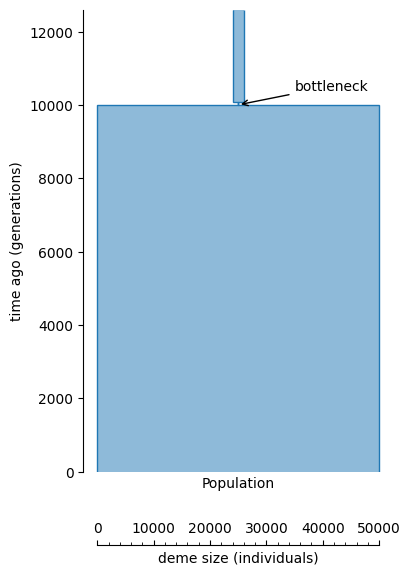
To illustrate this, we will generate data from a population that was large in recent history, but had a small bottleneck of only 100 individuals 10 thousand generations ago, lasting for (say) 80 generations, with a medium-sized population before that:
import msprime
import demesdraw
from matplotlib import pyplot as plt

bottleneck_time = 10000
demography = msprime.Demography()
demography.add_population(name="Population", initial_size=5e4)
demography.add_population_parameters_change(time=bottleneck_time, initial_size=100)
demography.add_population_parameters_change(time=bottleneck_time + 80, initial_size=2e3)

mutation_rate = 1e-8
# Simulate a short tree sequence with a population size history.
ts = msprime.sim_ancestry(
    10, sequence_length=2e6, recombination_rate=2e-8, demography=demography, random_seed=321)
ts = msprime.sim_mutations(ts, rate=mutation_rate, random_seed=321)
fig, ax = plt.subplots(1, 1, figsize=(4, 6))
demesdraw.tubes(demography.to_demes(), ax, scale_bar=True)
ax.annotate(
  "bottleneck",
  xy=(0, bottleneck_time),
  xytext=(1e4, bottleneck_time * 1.04),
  arrowprops=dict(arrowstyle="->"))
Text(10000.0, 10400.0, 'bottleneck')
To test how well tsdate does in this situation, we can redate the known (true) tree sequence topology, which replaces the true node and mutation times with estimates from the dating algorithm.
import tsdate
redated_ts = tsdate.date(ts, mutation_rate=mutation_rate, match_segregating_sites=True)
If we plot true node time against tsdate-estimated node time for each node in the tree sequence, we can see that the tsdate estimates are pretty much in line with the truth, although there is a a clear band which is difficult to date at 10,000 generations, corresponding to the instantaneous change in population size at that time.
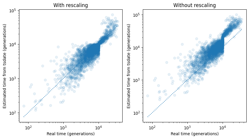
The plot on the right is from running tsdate without the rescaling step. It is clear that for populations with variable sizes over time, rescaling can help considerably in obtaining correct date estimations.
Misspecified priors#
Note
Functionality described below applies only to the non-default, Discrete-time methods, and is preliminary and subject to change in the future. For this reason, classes and methods may not form part of the publicly available API and may not be fully documented yet.
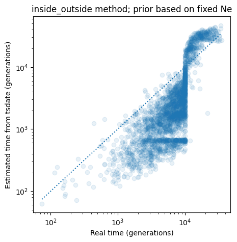
Approaches such as the inside_outside method that use a coalescent prior
based on a fixed population size. perform very poorly on data where
demography has been variable over time.
import tsdate
est_pop_size = ts.diversity() / (4 * mutation_rate)  # calculate av Ne from data
redated_ts = tsdate.inside_outside(ts, mutation_rate=mutation_rate, population_size=est_pop_size)
unconstr_times = [nd.metadata.get("mn", nd.time) for nd in redated_ts.nodes()]
fig, ax = plt.subplots(1, 1, figsize=(5, 5))
title = "inside_outside method; prior based on fixed Ne"
plot_real_vs_tsdate_times(ax, ts.nodes_time, unconstr_times, ts, redated_ts, alpha=0.1, title=title)
If you cannot use the variational_gamma method,
the discrete time methods also allow population_size to be either
a single number, specifying the “effective population size”,
or a piecewise constant function of time, specifying a set of fixed population sizes
over a number of contiguous time intervals. Functions of this sort are captured by the
PopulationSizeHistory class: see the Population size page
for its use and interpretation.
Estimating Ne for parameter specification#
In the example above, in the absence of an expected effective population size for use in the
inside_outside method, we used a value approximated from the data. The standard way to do so
is to use the (sitewise) genetic diversity divided by four-times the mutation rate:
print("A rough estimate of the effective population size is", ts.diversity() / (4 * 1e-6))
A rough estimate of the effective population size is 63.65526315789836