Tsinfer 0.3.0!
Tsinfer 0.3
Tsinfer 0.3.0 introduces a change to how inferred tree sequences are post-processed, which results in a substantial improvement in estimating dates for the oldest nodes in the tree sequence when running tsdate on inferred tree sequences. It also starts to lay groundwork for a more flexible system of inputting genetic data by allowing the genotypic allele index to be in any order, rather than requiring the ancestral allele to be first. Finally, changes are introduced to help avoid inappropriate downstream analyses (e.g. by setting time units and by removing topology in the flanks of the inferred tree sequence).
Brief summary of changes
1. Ancestral states do not need to correspond to genotype 0 (and can be inferred)
When creating a tsinfer input file, instead of the ancestral state being the first allele in the list, with value 0 in the associated genotypes array, you can now specify an “ancestral_allele” index and provide the alleles in any order. We can also provide an “ancestral_allele” of -1 (tskit.MISSING_DATA) which tells tsinfer to places mutations at that site using parsimony, inferring a parsimonious ancestral state.
import tsinfer
import tskit
from tskit import MISSING_DATA

with tsinfer.SampleData(sequence_length=100) as sd:
    sd.add_site(51, [1, 0, 1, 1, 1], ["A", "T"], ancestral_allele=1)  # Anc allele is "T"
    sd.add_site(52, [0, 0, 0, 1, 1], ["G", "C"], ancestral_allele=0)
    sd.add_site(53, [0, 1, 1, 1, 0], ["C", "A"], ancestral_allele=0)
    sd.add_site(54, [0, 1, 1, 1, 1], ["G", "C"], ancestral_allele=MISSING_DATA)
    sd.add_site(55, [0, 1, 1, 1, 0], ["A", "C"], ancestral_allele=0)
    sd.add_site(56, [0, 1, 2, 0, 0], ["T", "G", "C"], ancestral_allele=0)

ts = tsinfer.infer(sd)
print("Ancestral state at site at position 51 is", ts.site(position=51).ancestral_state)
print("Ancestral state at site at position 54 inferred to be", ts.site(position=54).ancestral_state)
Ancestral state at site at position 51 is T
Ancestral state at site at position 54 inferred to be C
Plottting the mutations on the tree also reveals which alleles are ancestral
ts.draw_svg(
    size=(700, 300),
    y_axis=True,
    mutation_labels={m.id: f"{s.id}: {s.ancestral_state}→{m.derived_state}" for s in ts.sites() for m in s.mutations},
)

2. Inferred tree sequences have empty regions before the first and after the last site
In the plot above, the X scale goes from 51 to 57 (corresponding to the site positions 50-56). Previous versions of tsinfer created genalogies that spanned the
entire genome (i.e 0..100 in this example). In tsinfer 0.3, the post-processing step (see 4. below) erases flanking regions, i.e. those before the first site position, or after the last site position plus one. By default, empty flanking regions are not plotted, but you can see them by explicitly setting the x limits to the full genome:
ts.draw_svg(size=(700, 300), x_lim=(0, ts.sequence_length), y_axis=True)

Note that this change affects the number of trees reported:
print(ts.num_trees, "trees in the tree sequence") # 4, not 2, because the empty regions count as trees!
4 trees in the tree sequence
You may have to adjust your code to account for the fact that the first and last trees may be empty. For instance, to plot the tMRCAs between 3 and 4 across the tree sequence, you will need something like this:
for tree in ts.trees():
    if tree.num_roots != ts.num_samples:
        # this is not an empty tree - mrca calculations will fail on an empty tree
        print(f"MRCA of 3 and 4 in the {tree.interval} is at time {tree.tmrca(3,4)}")
MRCA of 3 and 4 in the Interval(left=51.0, right=53.0) is at time 0.4
MRCA of 3 and 4 in the Interval(left=53.0, right=57.0) is at time 0.8999999999999999
3. Inferred tree sequence time units are set to “uncalibrated”
In the plot above, the time scale is labelled as “uncalibrated”. This means that attmepting to calculate statistics using branch lengths will raise an error, rather than (as previously) producing a meaningless value:
print(f"Time units in the inferred tree sequence are set to '{ts.time_units}'")
print("Sitewise diversity =", ts.diversity())  # This is OK as it isn't calculated form branch lengths
print(ts.diversity(mode="branch"))  # This now fails
Time units in the inferred tree sequence are set to 'uncalibrated'
Sitewise diversity = 0.033


---------------------------------------------------------------------------

LibraryError                              Traceback (most recent call last)

<ipython-input-6-7e58b3492861> in <module>
      1 print(f"Time units in the inferred tree sequence are set to '{ts.time_units}'")
      2 print("Sitewise diversity =", ts.diversity())  # This is OK as it isn;t calculated form branch lengths
----> 3 print(ts.diversity(mode="branch"))  # This now fails


/usr/local/lib/python3.9/site-packages/tskit/trees.py in diversity(self, sample_sets, windows, mode, span_normalise)
   7475             If there is one sample set and windows=None, a numpy scalar is returned.
   7476         """
-> 7477         return self.__one_way_sample_set_stat(
   7478             self._ll_tree_sequence.diversity,
   7479             sample_sets,


/usr/local/lib/python3.9/site-packages/tskit/trees.py in __one_way_sample_set_stat(self, ll_method, sample_sets, windows, mode, span_normalise, polarised)
   7350
   7351         flattened = util.safe_np_int_cast(np.hstack(sample_sets), np.int32)
-> 7352         stat = self.__run_windowed_stat(
   7353             windows,
   7354             ll_method,


/usr/local/lib/python3.9/site-packages/tskit/trees.py in __run_windowed_stat(self, windows, method, *args, **kwargs)
   7312         strip_dim = windows is None
   7313         windows = self.parse_windows(windows)
-> 7314         stat = method(*args, **kwargs, windows=windows)
   7315         if strip_dim:
   7316             stat = stat[0]


LibraryError: Statistics using branch lengths cannot be calculated when time_units is 'uncalibrated'. (TSK_ERR_TIME_UNCALIBRATED)
4. Post processing
The largest change in tsinfer 0.3 is the replacement of “simplification” with a more general “post-processing” step, which tweaks the tree sequence in various ways before simplifying. In particular the new tsinfer.post_process() routine, which is normally called automatically as the final step of inference, does the following by default:
- Removes the single ancestor that tsinfer has inserted (for technical reasons) above the “ultimate ancestor”
- Cuts up the ultimate ancestral node (consisting of entirely ancestral states) into separate chunks.
- Erases tree topology that exists before the first site and one unit after the last site (see 2. above)
- As before, “simplifies” the tree sequence (keeping unary nodes and re-allocating node ids so that the sample nodes have the same IDs as in the original sample data file)
To demonstrate, here’s a simulated dataset:
import msprime
import tsinfer
import matplotlib.pyplot as plt
import numpy as np

rho = 1e-7
mu = 10 * rho
Ne = 5e3
filename = "simulated_data.samples"
ts = msprime.sim_ancestry(
    10,
    sequence_length=10000,
    population_size=Ne,
    recombination_rate=rho,
    random_seed=333
)
ts = msprime.sim_mutations(ts, rate=mu, random_seed=333)
print("Simulated", ts.num_trees, "trees", ts.num_sites, "sites")
sample_data = tsinfer.SampleData.from_tree_sequence(ts, path=filename)
print(f"Saved genetic variation to '{filename}'")
Simulated 58 trees 682 sites
Saved genetic variation to 'simulated_data.samples'
Below we plot a portion of this inferred tree sequence “simplified” in the same way as in previous tsinfer versions. For clarity, the parent of the ultimate ancestor, inserted for technical reasons, is marked as “X”
plot_region = (2e3, 3e3)
inferred_simplified_ts = tsinfer.infer(sample_data, simplify=True)
print("Default output in tsinfer version 0.2.3")
inferred_simplified_ts.simplify(range(10), keep_unary=True).draw_svg(
    size=(1000, 500),
    x_lim=plot_region,
    node_labels={85: "...", 89: 89, 90: 90, 91: "ultimate anc.", 92: "X"},
    mutation_labels={},
    time_scale="rank",
    style=".n91 > .lab, .n91 > .sym {fill: green}"
)
The `simplify` parameter is deprecated in favour of `post_process`


Default output in tsinfer version 0.2.3

inferred_postprocessed_ts = tsinfer.infer(sample_data)  # post-process happens by default
print("New output in tsinfer version 0.3:")
print(" ancestor X removed, and ultimate ancestor split into multiple nodes")
matplotlib_colours = {
    "tab:blue": "#1f77b4", "tab:orange": "#ff7f0e", "tab:green": "#2ca02c", "tab:red": "#d62728"
}
mpl_vals = list(matplotlib_colours.values())
inferred_postprocessed_ts.simplify(range(10), keep_unary=True).draw_svg(
    size=(1000, 500),
    x_lim=(2e3, 3e3),
    time_scale="rank",
    node_labels={85: "...", 89: 89, 90: 90, 91: 91, 92: 92, 93: 93, 94: 94},
    mutation_labels={},
    style="".join([
        f".n{u}>.lab, .n{u}>.sym" + "{fill: " + mpl_vals[i] + "}"
        for i, u in enumerate(range(91, 95))
    ]),
)
New output in tsinfer version 0.3:
 ancestor X removed, and ultimate ancestor split into multiple nodes

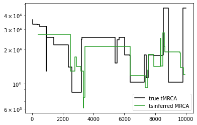
The rationale for splitting the ultimate ancestor is that we expect there to be multiple ancestors representing haplotypes with entirely ancestral states. As a heuristic, the ultimate ancestor is split whenever its children change. Although it makes no difference to the inferred topology, splitting the ultimate ancestor can result in a considerable improvement in the dates of the oldest nodes when dating the tree sequence:
import tsdate
mrcas_orig = [[t.interval.right, t.time(t.root)] for t in ts.trees()]

new_inferred_ts = inferred_postprocessed_ts.simplify()  # remove unary nodes for tsdate
dated_postprocessed_ts = tsdate.date(inferred_ts, mutation_rate=mu, Ne=Ne)
mrcas_new_method = [
    [t.interval.right, t.time(t.root)]
    for t in dated_postprocessed_ts.trees()
    if t.num_roots != dated_postprocessed_ts.num_samples
]

plt.step(*np.array(mrcas_orig).T, c="black", label="true tMRCA")
plt.step(*np.array(mrcas_new_method).T, c="tab:green", label="tsinferred MRCA")
plt.legend()
plt.yscale("log")
old_inferred_simplified_ts = inferred_simplified_ts.simplify() # remove unary nodes
dated_simplified_ts = tsdate.date(old_inferred_simplified_ts, mutation_rate=mu, Ne=Ne)
mrcas_old_method = [
[t.interval.right, t.time(t.root)]
for t in dated_simplified_ts.trees()
if t.num_roots != dated_simplified_ts.num_samples
]
mrcas_old = [
[t.interval.right, t.time(t.root)]
for t in dated_simplified_ts.trees()
if t.num_roots != dated_simplified_ts.num_samples
]
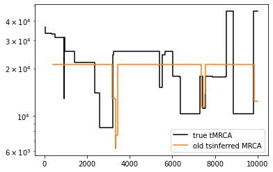
plt.step(*np.array(mrcas_orig).T, c="black", label="true tMRCA")
plt.step(*np.array(mrcas_old).T, c="tab:orange", label="old tsinferred MRCA")
plt.legend()
plt.yscale("log")
5. Command line interface (CLI) improvements
For large inferences, we recommend running tsinfer on the command-line, e.g.
! python3 -m tsinfer generate-ancestors simulated_data.samples
This CLI interface now allows the mismatch ratio and recombination rate to be specified. Alternatively, the path to a recombination map in hapmap format (as read by msprime.RateMap.read_hapmap) can be given:
! python3 -m tsinfer infer --recombination_rate=0.4 --mismatch_ratio=0.1 simulated_data.samples -O inferred.ts
# Or python3 -m tsinfer infer --recombination_map=/path/to/hapmap --mismatch_ratio=0.1 simulated_data.samples
These parameters are saved to the provenance of the output tree sequence
import json
inferred_ts = tskit.load("inferred.ts")
print(json.loads(inferred_ts.provenance(-1).record)["parameters"])
{'args': ['infer', '--recombination_rate=0.4', '--mismatch_ratio=0.1', 'simulated_data.samples', '-O', 'inferred.ts'], 'command': '/Users/yan/Documents/GitHub/tsinfer/tsinfer/__main__.py'}
6. Misc changes
- The CLI allows
--no-post-processto be specified when matching samples
! python3 -m tsinfer match-ancestors simulated_data.samples
! python3 -m tsinfer match-samples --no-post-process simulated_data.samples -O simulated_no_pp.trees
- If we want to post-process afterwards, there is a separate routine,
tsinfer.post_process()which accepts extra options e.g. to avoid splitting the ultimate ancestor or erasing topology in flanking regions:
no_pp_ts = tskit.load("simulated_no_pp.trees")
pp_ts = tsinfer.post_process(no_pp_ts, split_ultimate=False, erase_flanks=False)
- matching routines warn if no inference sites have been used:
ancestors = tsinfer.generate_ancestors(sd, exclude_positions=[s.position for s in sd.sites()])
anc_ts = tsinfer.match_ancestors(sd, ancestors)
No sites used for inference
sample_data.subset()now accepts a sequence_length
shorter_sample_data = sample_data.subset(
    sites=range(100),
    sequence_length=sample_data.sites_position[:][101])
print("Original data covers ", sample_data.sequence_length, "bp")
print("Subset covers ", shorter_sample_data.sequence_length, "bp")
Original data covers  10000.0 bp
Subset covers  1098.0 bp
verifyno longer raises error when comparing a genotype to missingness (see issue 625)
Feedback etc
Please post a discussion or an issue on the tsinfer GitHub repository if you have any problems. We hope the update to tsinfer version 0.3 is useful in your research.