Large scale inference (legacy)#
Warning
This page documents the old Python batch matching API which is no longer the recommended workflow. It is retained as a reference while the content is ported to the new TOML config + CLI interface described in the quickstart.
Generally, for up to a few thousand samples a single multi-core machine can infer a tree sequence in a few days, hours, or even minutes. However, tsinfer has been successfully used with datasets up to half a million samples, where ancestor and sample matching can take several CPU-years. At this scale inference must be scaled across many machines. Tsinfer provides specific APIs to enable this. Here we detail considerations and tips for each step of the inference process to help you scale up your analysis. A snakemake pipeline which implements this parallelisation scheme is available as tsinfer-snakemake.
Data preparation#
For large scale inference the data must be in VCF Zarr
format, read by the VariantData class. Bio2zarr
is recommended for conversion from VCF, and sgkit can then
be used to perform initial filtering.
Todo
An upcoming tutorial will detail conversion from VCF to a VCF Zarr suitable for tsinfer.
Ancestor generation#
Ancestor generation is generally the fastest step in inference. It is not yet
parallelised out-of-core in tsinfer and must be performed on a single machine.
However it scales well on machines with
many cores and hyperthreading via the num_threads argument to
generate_ancestors. The limiting factor is often that the
entire genotype array for the contig being inferred needs to fit in RAM.
This is the high-water mark for memory usage in tsinfer.
If your data consists of only biallelic sites, with no missingness,
the genotype_encoding argument can be set to
GenotypeEncoding.ONE_BIT which reduces the memory footprint of
the genotype array by a factor of 8, such that the RAM needed is roughly
num_sites * num_samples * ploidy / 8 bytes. This memory optimisation
results in a surprisingly small increase in runtime.
Ancestor matching#
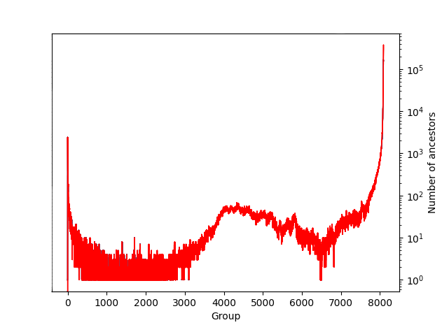
Ancestor matching is one of the more time consuming steps of inference. It proceeds in groups, progressively growing the tree sequence with younger ancestors. At each stage the parallelism is limited to the number of ancestors whose possible inheritors are already matched, as all possible inheritors of a sample must be matched in an earlier group. For a typical human data set the number of samples per group varies from single digits up to approximately the number of samples. The plot below shows the number of ancestors matched in each group for a typical human data set, earlier groups are older ancestors:
There are five tsinfer API methods that can be used to parallelise ancestor matching.
The five methods are:
match_ancestors_batch_initmatch_ancestors_batch_groupsmatch_ancestors_batch_group_partitionmatch_ancestors_batch_group_finalisematch_ancestors_batch_finalise
Initially match_ancestors_batch_init should be called to
set up the batch matching and to determine the groupings of ancestors.
This method writes a file metadata.json to the work_dir that contains
a JSON encoded dictionary with configuration for later steps, and a key
ancestor_grouping which is a list of dictionaries, each containing the
list of ancestors in that group (key:ancestors) and a proposed partioning of
those ancestors into sets that can be matched in parallel (key:partitions).
The dictionary is also returned by the method.
The partitioning is controlled by the min_work_per_job and max_num_partitions
arguments. For each group, ancestors are placed in a partition until the sum of their
lengths exceeds min_work_per_job, when a new partition is started. However, the
number of partitions is not allowed to exceed max_num_partitions. It is suggested
to set max_num_partitions to around 3-4x the number of worker nodes available,
and min_work_per_job to around 2,000,000 for a typical human data set.
Groups vs partitions is a point of common confusion. Note that groups of ancestors are matched serially, and each group is split into partitions that can be matched in parallel.
Each group is matched in turn, either by calling match_ancestors_batch_groups
to match without partitioning, or by calling match_ancestors_batch_group_partition
many times in parallel followed by a single call to match_ancestors_batch_group_finalise.
Each call to match_ancestors_batch_groups or match_ancestors_batch_group_finalise
outputs the tree sequence to work_dir, which is then used by the next group. The length of
the ancestor_grouping in the metadata dictionary determines the group numbers that these methods
will need to be called for, and the length of the partitions list in each group determines
the number of calls to match_ancestors_batch_group_partition that are needed (if any).
match_ancestors_batch_groups matches groups, without partitioning, from
group_index_start (inclusively) to group_index_end (exclusively). Combining
many groups into one call reduces the overhead from job submission and start
up times, but note on job failure the process can only be resumed from the
last group_index_end.
To match a single group in parallel, call match_ancestors_batch_group_partition
once for each partition listed in the ancestor_grouping[group_index]['partitions'] list,
incrementing partition_index. This will match the ancestors, placing the match data in
the working_dir. Once all are complete a single call to
match_ancestors_batch_group_finalise will then insert the matches and
output the tree sequence to work_dir.
Each call to match_ancestors_batch_groups and match_ancestors_batch_group_finalise results in a tree sequence being written to work_dir.
These tree sequences are essentially checkpoints from with the batch matching workflow
can be resumed on job failure.
Finally after the final group, call match_ancestors_batch_finalise to
combine the groups into a single tree sequence.
The partitioning in metadata.json does not have to be used for every group. As early groups are
not matching to a large tree sequence it is often faster to not partition the first half of the
groups, depending on job set up and queueing time on your cluster.
Calls to match_ancestors_batch_group_partition will only use a single core, but
match_ancestors_batch_groups will use as many cores as num_threads is set to.
Therefore this value and cluster resources requested should be scaled with the number of ancestors,
which can be read from the metadata dictionary.
As an example of how the API methods can be used together, suppose the metadata dictionary
created by match_ancestors_batch_init contains the following:
{
    "ancestor_grouping": [
        {"ancestors": [0, ... 9], "partitions": None},
        {
          "ancestors": [10, ... 15],
          "partitions": [[10, 11, 12], [13, 14, 15]]
        },
        {"ancestors": [16, ... 19], "partitions": None},
        {"ancestors": [20, ... 25], "partitions": None},
        {"ancestors": [26, ... 30], "partitions": None},
        {
          "ancestors": [31, ... 41],
          "partitions": [[31, 32, 33, 34, 35, 36], [37, 38, 39, 40, 41]]
        },
        {"ancestors": [42, ... 45], "partitions": None},
        {"ancestors": [46, ... 50], "partitions": None},
        {
          "ancestors": [51, ... 65],
          "partitions": [
            [51, 52, 53, 54],
            [55, 56, 57, 58],
            [59, 60, 61, 62, 63, 64, 65]
          ]
        },
    ]
}
Then the flow could look like the following diagram: (calls on the same horizontal line can be done in parallel, note that method names are shortened):

Note that groups 1, 5 and 8 can be partitioned, but only groups 5 and 8 are actually partitioned in this example, as stated above partitioning for groups is optional. Groups 0-4 are matched in one call, groups 6 and 7 are matched in two calls, but could have been matched in one. By splitting 6 and 7 the flow makes an additional resume point in the case of job failure at the cost of job start up and queueing time.
Sample matching#
Sample matching is far simpler than ancestor matching as it is essentially the same as a single group of ancestors. There are three API methods that work together to enable distributed sample matching.
match_samples_batch_initmatch_samples_batch_partitionmatch_samples_batch_finalise
match_samples_batch_init should be called to set up the batch matching and to determine the
groupings of samples. Similar to match_ancestors_batch_init it has a min_work_per_job argument to control the level of parallelism. The method writes a file
metadata.json to the directory work_dir that contains a JSON encoded dictionary with
configuration for later steps. This is also returned by the call. The num_partitions key in
this dictionary is the number of times match_samples_batch_partition will need
to be called, with each partition index as the partition_index argument. These calls can happen
in parallel and write match data to the work_dir which is then used by
match_samples_batch_finalise to output the tree sequence.