Tutorial#
This tutorial covers the most common uses of tree sequences in SLiM/pyslim.
Recapitation, simplification, and mutation#
Perhaps the most common pyslim operations involve Recapitation, Simplification, and/or Adding neutral mutations to a SLiM simulation. Below we illustrate all three in the context of running a “hybrid” simulation, combining both forwards and backwards (coalescent) methods. This hybrid approach is a popular application of pyslim because coalescent algorithms, although more limited in the degree of biological realism they can attain, can be much faster than the forwards algorithms implemented in SLiM.
A typical use-case is to take an existing SLiM simulation and endow it with a history derived from a coalescent simulation: this is known as recapitation. For instance, suppose we have a SLiM simulation of a population of 100,000 individuals that we have run for 10,000 generations without neutral mutations. Now, we wish to extract whole-genome genotype data for only 1,000 individuals. Here’s one way to do it:
recapitate(): The simulation has likely not reached demographic equilibrium - it has not coalesced entirely; recapitation uses coalescent simulation to provide a “prior history” for the initial generation of the simulation.simplify(): For efficiency, subset the tree sequence to only the information relevant for those 1,000 individuals we wish to sample.msprime.sim_mutations(): Add neutral mutations to the tree sequence.
These steps are described below. First, to get something to work with, you can run this simple SLiM script of a single population of sexual organisms, fluctuating around 1000 individuals, for 1000 generations:
initialize() {
   initializeSLiMModelType("nonWF");
   initializeSex("A");
   initializeTreeSeq();
   initializeMutationRate(0.0);
   initializeMutationType("m1", 0.5, "f", 0.0);
   initializeGenomicElementType("g1", m1, 1.0);
   initializeGenomicElement(g1, 0, 1e8-1);
   initializeRecombinationRate(1e-8);
   defineConstant("K", 1000);
}

reproduction(p1, "F") {
   subpop.addCrossed(individual,
                     subpop.sampleIndividuals(1, sex="M"));
}

1 early() {
   sim.addSubpop("p1", K);
}

early() {
   p1.fitnessScaling = K / p1.individualCount;
}

1000 late() {
   sim.treeSeqOutput("example_sim.trees");
}
You can run this in the shell, setting the random seed so you get exactly the same results as in the code below:
%%bash
slim -s 23 example_sim.slim
Recapitation#
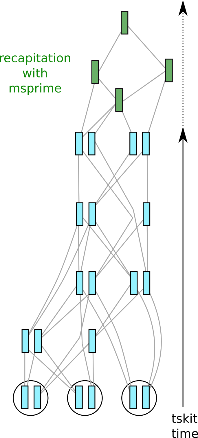
Fig. 4 Recapitation adds the green nodes by coalescent simulation. (See the introduction for a diagram of the previous state.)#
Although we can initialize a SLiM simulation with the results of a coalescent simulation, if during the simulation we don’t actually use the genotypes for anything, it can be much more efficient to do this afterwards, hence only doing a coalescent simulation for the portions of the first-generation ancestors that have not yet coalesced. (See the SLiM manual for more explanation.) This is depicted in figure 4: imagine that at some sites, some of the samples don’t share a common ancestor within the SLiMulated portion of history (shown in blue). Recapitation starts at the top of the genealogies, and runs a coalescent simulation back through time to fill out the rest of genealogical history relevant to the samples. The green chromosomes are new ancestral nodes that have been added to the tree sequence. This is important - if we did not do this, then effectively we are assuming the initial population would be genetically homogeneous, and so our simulation would have less genetic variation than it should have (since the component of variation from the initial population would be omitted).
Doing this is as simple as:
orig_ts = tskit.load("example_sim.trees")
rts = pyslim.recapitate(orig_ts,
            recombination_rate=1e-8,
            ancestral_Ne=200, random_seed=5)
The warning is harmless; it is reminding us to think about generation time when recapitating a nonWF simulation (a topic we’ll deal with later).
We can check that this worked as expected, by verifying that after recapitation all trees have only one root:
orig_max_roots = max(t.num_roots for t in orig_ts.trees())
recap_max_roots = max(t.num_roots for t in rts.trees())
print(f"Maximum number of roots before recapitation: {orig_max_roots}\n"
      f"After recapitation: {recap_max_roots}")
Maximum number of roots before recapitation: 13
After recapitation: 1
The recapitate() method
is just a thin wrapper around msprime.sim_ancestry(),
and you need to set up demography explicitly - for instance, in the example above
we’ve simulated from an ancestral population of Ne=200 diploids.
If you have more than one population,
you must set migration rates or else coalescence will never happen
(see Recapitation with migration between more than one population for an example,
and recapitate() for more).
Recapitation with a nonuniform recombination map#
Above, we recapitated using a uniform genetic map. But, msprime - like SLiM - can simulate with recombination drawn from an arbitrary genetic map. Let’s say we’ve already got a recombination map as specified by SLiM, as a vector of “positions” and a vector of “rates”. msprime also needs vectors of positions and rates, but the format is slightly different. To use the SLiM values for msprime, we need to do three things:
Add a 0 at the beginning of the positions,
add 1 to the last position.
The reason why msprime “positions” must start with 0 (step 1) is that in SLiM,
a position or “end” indicates the end of a recombination block such that its associated
“rate” applies to everything to the left of that end (see initializeRecombinationRate).
In msprime, we will pass in a msprime.RateMap,
which requires two things:
position: A list of n+1 positions, starting at 0, and ending in the sequence length over which the RateMap will apply.rate: A list of n positive rates that apply between each position.
So, msprime needs a vector of positions that is 1 longer than what you give SLiM, but one fewer rate values than positions.
The reason for step 2 is that intervals for tskit (which msprime uses) are “closed on the left and open on the right”, which means that the genomic interval from 0.0 to 100.0 includes 0.0 but does not include 100.0. If SLiM has a final genomic position of 99, then it could have mutations occurring at position 99. Such mutations would not be legal, on the other hand, if we set the tskit sequence length to 99, since the position 99 would be outside of the interval from 0 to 99. Said another way, if SLiM’s final position is 99, the total sequence length is 100, and so we need to set the end of the genome to 100. The upshot is that we need to use SLiM’s last position plus one - i.e., the length of the genome - as the rightmost coordinate.
For instance, suppose that we have a recombination map file in the following (tab-separated) format:
end_position	rate(cM/Mb)
15000000	3.2
50000000	2.5
85000000	0.25
99999999	2.8
This describes recombination rates across a 100Mb genome with higher rates on the ends (for instance, 3.2 and 2.8 cM/Mb in the first and last 15Mb respectively) and lower rates in the middle (0.25 cM/Mb between 50Mb and 85Mb). The first column gives the starting position, in bp, for the window whose recombination rate is given in the second column. (Note: this is not a standard format for recombination maps - it is more usual for the starting position to be listed!)
Here is SLiM code to read this file and set the recombination rates:
lines = readFile("recomb_rates.tsv");
header = strsplit(lines[0], "\t");
if (header[0] != "end_position"
    | header[1] != "rate(cM/Mb)") {
   stop("Unexpected format!");
}
rates = NULL;
ends = NULL;
nwindows = length(lines) - 1;
for (line in lines[1:nwindows]) {
  components = strsplit(line, "\t");
  ends = c(ends, asInteger(components[0]));
  rates = c(rates, asFloat(components[1]));
}
initializeRecombinationRate(rates * 1e-8, ends);
Now, here’s code to take the same recombination map used in SLiM, and use it for recapitation in msprime:
positions = []
rates = []
with open('_static/recomb_rates.tsv', 'r') as file:
  header = file.readline().strip().split("\t")
  assert(header[0] == "end_position" and header[1] == "rate(cM/Mb)")
  for line in file:
     components = line.split("\t")
     positions.append(float(components[0]))
     rates.append(1e-8 * float(components[1]))

# step 1
positions.insert(0, 0)
# step 2
positions[-1] += 1
assert positions[-1] == orig_ts.sequence_length

recomb_map = msprime.RateMap(position=positions, rate=rates)
rts = pyslim.recapitate(orig_ts,
                recombination_rate=recomb_map,
                ancestral_Ne=200, random_seed=7)
assert(max([t.num_roots for t in rts.trees()]) == 1)
(As before, you should not usually explicitly set the random seed in your scripts; we set it here so the content of this document does not change.)
Note
Starting from msprime 1.0, the default model of recombination in msprime is discrete - recombinations only occur at integer locations - which matches SLiM’s model of recombination.
Simplification#
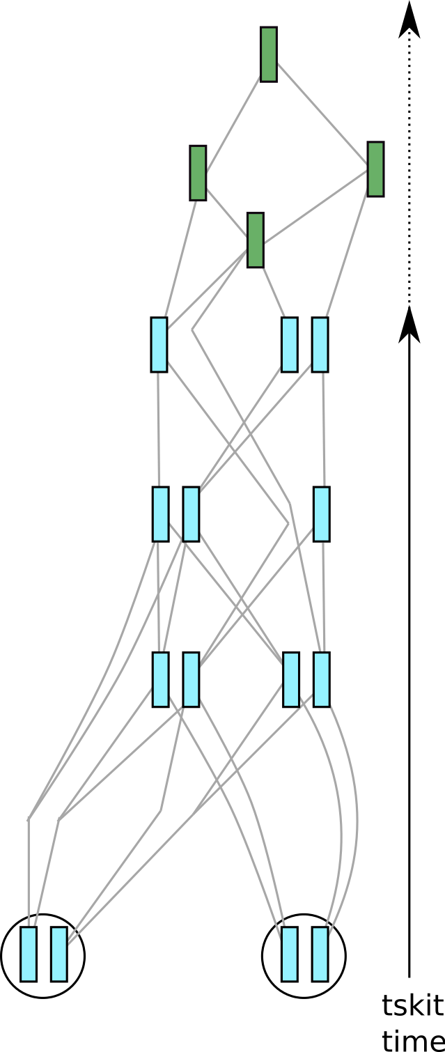
Fig. 5 The result of simplifying the tree sequence in figure figure 4 to only two of the three samples.#
Probably, your simulations have produced many more fictitious genomes than you will be lucky enough to have in real life, so at some point you may want to reduce your dataset to a realistic sample size. We can get rid of unneeded samples and any extra information from them by using an operation called simplification (this is the same basic approach that SLiM implements under the hood when outputting a tree sequence, as described in the introduction).
Depicted in the figure at the right is the result of applying an explicit call to
tskit.TreeSequence.simplify() to our example tree sequence.
In the call we asked to keep only 4
genomes (contained in 2 of the individuals in the current generation). This has
substantially simplified the tree sequence, because only information relevant to the
genealogies of the 4 sample nodes has been kept. (Precisely, simplification retains only
nodes of the tree sequence that are branching points of some marginal genealogy – see
Kelleher et al 2018 for details.)
While simplification sounds very appealing - it makes things simpler after all -
it is often not necessary in practice, because tree sequences are very compact,
and many operations with them are quite fast.
(It will, however, speed up many operations, so if you plan to do a large number of simulations,
your workflow could benefit from early simplification.)
So, you should probably not make simplification a standard step in your workflow,
only using it if necessary.
It is important that simplification - if it happens at all -
either (a) comes after recapitation, or (b) is done with the
keep_input_roots=True option (see tskit.TreeSequence.simplify()).
This is because simplification removes some of the
ancestral genomes in the first generation,
which are necessary for recapitation,
unless it is asked to “keep the input roots”.
If we simplify without this option before recapitating,
some of the first-generation blue chromosomes in the figure on the right
would not be present, so the coalescent simulation would start from a more recent point in time
than it really should.
As an extreme example, suppose our SLiM simulation has a single diploid who has reproduced
by clonal reproduction for 1,000 generations,
so that the final tree sequence is just two vertical lines of descent going back
to the two chromosomes in the initial individual alive 1,000 generations ago.
Recapitation would produce a shared history for these two chromosomes,
that would coalesce some time longer ago than 1,000 generations.
However, if we simplified first, then those two branches going back 1,000 generations would be removed,
since they don’t convey any information about the shape of the tree;
and so recapitation might produce a common ancestor more recently than 1,000 generations,
which would be inconsistent with the SLiM simulation.
After recapitation,
simplification to the history of 100 individuals alive today
can be done with the tskit.TreeSequence.simplify() method:
import numpy as np
rng = np.random.default_rng(seed=3)
alive_inds = pyslim.individuals_alive_at(rts, 0)
keep_indivs = rng.choice(alive_inds, 100, replace=False)
keep_nodes = []
for i in keep_indivs:
  keep_nodes.extend(rts.individual(i).nodes)

sts = rts.simplify(keep_nodes, keep_input_roots=True)

print(f"Before, there were {rts.num_samples} sample nodes (and {rts.num_individuals} individuals)\n"
      f"in the tree sequence, and now there are {sts.num_samples} sample nodes\n"
      f"(and {sts.num_individuals} individuals).")
Before, there were 1960 sample nodes (and 980 individuals)
in the tree sequence, and now there are 200 sample nodes
(and 118 individuals).
Note that you must pass simplify a list of node IDs, not individual IDs.
Here, we used the individuals_alive_at() method to obtain the list
of individuals alive today.
Also note that there are still more than 100 individuals remaining - 15 non-sample individuals
have not been simplified away,
because they have nodes that are required to describe the genealogies of the samples.
(Since this is a non-Wright-Fisher simulation,
parents and children can be both alive at the same time in the final generation.)
Adding neutral mutations to a SLiM simulation#
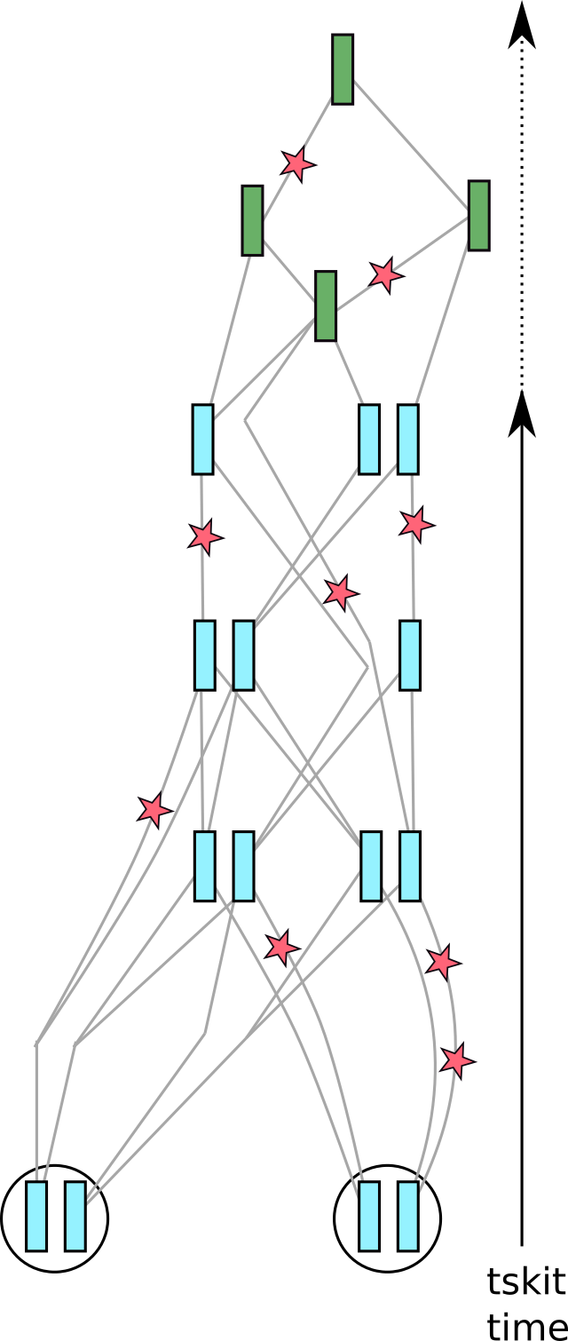
Fig. 6 The tree sequence, with mutations added.#
If you have recorded a tree sequence in SLiM, likely you have not included any neutral mutations,
since it is much more efficient to simply add these on afterwards.
To add these (in a completely equivalent way to having included them during the simulation),
you can use the msprime.sim_mutations() function, which returns a new tree sequence with additional mutations.
Continuing with the cartoons from above, these are added to each branch of the tree sequence
at the rate per unit time that you request.
We’ll add these using the msprime.SLiMMutationModel, so that the file can be read back into SLiM,
but any of the other mutation models in msprime could be used.
This works as follows:
next_id = pyslim.next_slim_mutation_id(sts)
ts = msprime.sim_mutations(
           sts,
           rate=1e-8,
           model=msprime.SLiMMutationModel(type=0, next_id=next_id),
           keep=True,
)

print(f"The tree sequence now has {ts.num_mutations} mutations,\n"
      f"and mean pairwise nucleotide diversity is {ts.diversity():0.3e}.")
The tree sequence now has 27281 mutations,
and mean pairwise nucleotide diversity is 2.333e-05.
What’s going on here? Let’s step through the code.
The mutation
rate = 1e-8, which adds mutations at a rate of \(10^{-8}\) per bp. Unlike previous versions of msprime, this adds mutations using a discrete-sites model, i.e., only at integer locations (like SLiM).We’re passing
type=0to the mutation model. This is because SLiM mutations need a “mutation type”, and it makes the most sense if we add a type that was unused in the simulation. In this example we don’t have any existing mutation types, so we can safely usetype=0.We also add
keep = True, to keep any existing mutations. In this example there aren’t any, so this isn’t strictly necessary, but this is a good default.If there are existing SLiM mutations on the tree sequence we need to make sure any newly added mutations have distinct SLiM IDs, so we use
next_slim_mutation_id()to figure out what the next available ID is, and pass it in.
Writing out genotypes to VCF#
Downstream applications often need input in VCF format,
which we can get with a call to tskit.TreeSequence.write_vcf().
However, if we do that with this tree sequence, we’ll get a malformed VCF,
with empty strings in the REF column and a strange comma-separated list of integers
in the ALT column. The reason for this is because we added mutations
using the SLiMMutationModel, and has to do with how SLiM stores enough information
in the tree sequence to be able to load it back in.
So, to write out valid VCF with nucleotides for alleles,
we need to (1) if the SLiM simulation was not a nucleotide model, add nucleotides
to the SLiM mutations with generate_nucleotides(),
and (2) move those nucleotides over into the “ancestral state”
and “derived state” slots of the tree sequence with convert_alleles().
If all your mutations in SLiM were nucleotide mutations, you only need to do (2).
And, beware that (2) is an irreversible step: if you write the tree sequence
produced by convert_alleles() to a file, you can’t load that file into SLiM any more.
So, to do this we’ll do:
nts = pyslim.generate_nucleotides(ts)
nts = pyslim.convert_alleles(nts)
sample_indivs = np.unique([ts.node(n).individual for n in nts.samples()])
with open("example_sim.vcf", "w") as vcffile:
    nts.write_vcf(vcffile, individuals=sample_indivs[:5])
Here we’ve just extracted genotypes for the first five individuals;
see below for what’s going on in that code and what you probably
actually want to do;
see also tskit.TreeSequence.write_vcf() for more options.
Extracting SLiM individuals#
Another important thing to be able to do is to extract individuals from a simulation, for analysis or for outputting their genotypes, for instance. This section demonstrates some basic manipulations of individuals.
Extracting a sample of individuals#
The first, most common method to extract individuals is simply to get all
those that were alive at a particular time,
using individuals_alive_at(). For instance, to get
the list of individual IDs of all those alive at the end of the
simulation (i.e., zero time units ago), we could do:
orig_ts = tskit.load("example_sim.trees")
alive = pyslim.individuals_alive_at(orig_ts, 0)

print(f"There are {len(alive)} individuals alive in the final generation.")
There are 980 individuals alive in the final generation.
Here, alive is a vector of individual IDs,
so one way to take a sample of living individuals
and write their SNPs to a VCF is:
rng = np.random.default_rng(seed=1)
keep_indivs = rng.choice(alive, 100, replace=False)
ts = msprime.sim_mutations(orig_ts, rate=1e-8, random_seed=1)
with open("example_snps.vcf", "w") as vcffile:
    ts.write_vcf(vcffile, individuals=keep_indivs)
If you’ve done nothing else to the output from SLiM, then this code will work, but it does requires all alive individuals to be samples. A situation in which this isn’t the case is shown in the next section.
Extracting individuals after simplification#
If the tree sequence has been simplified to retain only information
about a set of focal individuals,
then knowing an individual is alive at the end of the simulation
isn’t enough to guarantee we have their entire genome sequence:
there are often individuals retained after simplification with
one or more non-sample nodes.
So, to output genotypes after simplification, we need to also check
that the individuals’ nodes are also samples.
As mentioned earlier, tskit.TreeSequence.simplify() takes a list
of nodes as input:
keep_nodes = []
for i in keep_indivs:
    keep_nodes.extend(orig_ts.individual(i).nodes)
sts = rts.simplify(keep_nodes)
ts = msprime.sim_mutations(sts, rate=1e-8, random_seed=1)
Individuals are retained by simplify if any of their nodes are, so we would get an alive individual without sample nodes if, for instance, a parent and two offspring are all alive, and we happen to keep the offspring but not the parent. For this reason, if at this point we try to extract genotypes for all of the alive individuals, we encounter a (somewhat confusing) error:
try:
    alive = pyslim.individuals_alive_at(ts, 0)
    with open("example_snps.vcf", "w") as vcffile:
        ts.write_vcf(vcffile, individuals=alive)
except Exception as e:
    print ("Error:")
    print (e)
This is just telling us that some of the individuals we’re trying
to write to the VCF have nodes that are not samples.
The reference to “missing” is a red herring:
see tskit documentation
for what it’s talking about.
So, instead of writing out genotypes of everyone alive,
we need to get the list of alive individuals whose nodes are samples,
using is_sample():
indivlist = []
for i in pyslim.individuals_alive_at(ts, 0):
    ind = ts.individual(i)
    if ts.node(ind.nodes[0]).is_sample():
       indivlist.append(i)
       # if one node is a sample, the other should be also:
       assert ts.node(ind.nodes[1]).is_sample()
with open("example_snps.vcf", "w") as vcffile:
    ts.write_vcf(vcffile, individuals=indivlist)
Extracting particular individuals#
Now let’s see how to examine other attributes of individuals, e.g., which subpopulation they’re in. To get another example with discrete subpopulations, let’s run another SLiM simulation, similar to the above but with two populations exchanging migrants:
initialize() {
   initializeSLiMModelType("nonWF");
   initializeSex("A");
   initializeTreeSeq();
   initializeMutationRate(0.0);
   initializeMutationType("m1", 0.5, "f", 0.0);
   initializeGenomicElementType("g1", m1, 1.0);
   initializeGenomicElement(g1, 0, 1e8-1);
   initializeRecombinationRate(1e-8);
   defineConstant("K", 1000);
}

reproduction(NULL, "F") {
   subpop.addCrossed(individual,
                     subpop.sampleIndividuals(1, sex="M"));
}


1 early() {
   sim.addSubpop("p1", K);
   sim.addSubpop("p2", K);
}

early() {
   num_migrants = rpois(2, 0.01 * c(p1.individualCount, p2.individualCount));
   migrants1 = sample(p1.individuals, num_migrants[0]);
   migrants2 = sample(p2.individuals, num_migrants[1]);
   p2.takeMigrants(migrants1);
   p1.takeMigrants(migrants2);
   p1.fitnessScaling = K / p1.individualCount;
   p2.fitnessScaling = K / p2.individualCount;
}

1000 late() {
   sim.treeSeqOutput("migrants.trees");
}
Let’s run it:
%%bash
slim -s 32 migrants.slim
To count up how many individuals are in each population, we could do:
orig_ts = tskit.load("migrants.trees")
alive = pyslim.individuals_alive_at(orig_ts, 0)
num_alive = [0 for _ in range(orig_ts.num_populations)]
for i in alive:
  ind = orig_ts.individual(i)
  ind_population = orig_ts.node(ind.nodes[0]).population
  num_alive[ind_population] += 1

for pop, num in enumerate(num_alive):
  print(f"Number of individuals in population {pop}: {num}")
Number of individuals in population 0: 0
Number of individuals in population 1: 1008
Number of individuals in population 2: 1015
Note
Our SLiM script started numbering populations at 1, while tskit starts counting at 0, so there is an empty “population 0” in a SLiM-produced tree sequence.
Recapitation with migration between more than one population#
Following on the last example,
let’s recapitate and mutate the tree sequence.
Recall that this recipe had two populations, p1 and p2,
each of size 1000.
Recapitation takes a bit more thought, because if the two populations stay separate,
it will run forever, unable to coalesce.
By default, recapitate() merges the two populations into a single
one of size ancestral_Ne.
But, if we’d like them to stay separate, we need to inclue migration between them.
Here’s how we set up the demography using msprime’s tools:
demography = msprime.Demography.from_tree_sequence(orig_ts)
for pop in demography.populations:
    # must set their effective population sizes
    pop.initial_size = 1000

demography.add_migration_rate_change(
    time=orig_ts.metadata['SLiM']['tick'],
    rate=0.1, source="p1", dest="p2",
)
demography.add_migration_rate_change(
    time=orig_ts.metadata['SLiM']['tick'],
    rate=0.1, source="p2", dest="p1",
)
rts = pyslim.recapitate(
        orig_ts, demography=demography,
        recombination_rate=1e-8,
        random_seed=4
)
ts = msprime.sim_mutations(
                    rts, rate=1e-8,
                    model=msprime.SLiMMutationModel(type=0),
                    random_seed=7
)
Again, there are three populations because SLiM starts counting at 1; the first population is unused (no migrants can go to it). Let’s compute genetic diversity within and between each of the two populations (we compute the mean density of pairwise nucleotide differences, often denoted \(\pi\) and \(d_{xy}\)). To do this, we need to extract the node IDs from the individuals of the two populations that are alive at the end of the simulation.
pop_nodes = [ts.samples(population=p, time=0) for p in range(ts.num_populations)]
diversity = ts.diversity(pop_nodes[1:])
divergence = ts.divergence(pop_nodes[1:])

print(f"There are {ts.num_mutations} mutations across {ts.num_trees} distinct\n"
      f"genealogical trees describing relationships among {ts.num_samples}\n"
      f"sampled genomes, with a mean genetic diversity of {diversity[0]:0.3e}\n"
      f"and {diversity[1]:0.3e} within the two populations,\n"
      f"and a mean divergence of {divergence:0.3e} between them.")
There are 114963 mutations across 51461 distinct
genealogical trees describing relationships among 4046
sampled genomes, with a mean genetic diversity of 9.013e-05
and 9.029e-05 within the two populations,
and a mean divergence of 9.089e-05 between them.
Individual metadata#
Each Mutation, Population, Node, and Individual, as well as the tree
sequence as a whole, carries additional information stored by SLiM in its metadata
property. A fuller description of metadata in general is given in Metadata,
but as a quick introduction, here is the information available
about an individual in the previous example:
ind = ts.individual(0)
Individual(id=0, flags=65536, location=array([0., 0., 0.]), parents=array([-1, -1], dtype=int32), nodes=array([11145, 11146], dtype=int32), metadata={
    'pedigree_id': 980494,
    'pedigree_p1': 974787,
    'pedigree_p2': 966513,
    'age': 21,
    'subpopulation': 1,
    'sex': 0,
    'flags': 0
   })
Some information is generic to individuals in tree sequences of any format:
id (the ID internal to the tree sequence),
flags (described below),
location (the [x,y,z] coordinates of the individual),
nodes (an array of the node IDs that represent the genomes of this individual),
and time (the time, in units of “time ago” that the individual was born).
Other information, contained in the metadata field, is specific to tree sequences
produced by SLiM. This is described in more detail in the SLiM manual, but briefly:
the
pedigree_idis SLiM’s internal ID for the individual,ageandsubpopulationare their age and population at the time they were recorded, or at the time the simulation stopped if they were still alive (NB: SLiM uses the word “subpopulation” for what is simply called a “population” in tree-sequence parlance)sexis their sex (as an integer, one ofINDIVIDUAL_TYPE_FEMALE,INDIVIDUAL_TYPE_MALE, orINDIVIDUAL_TYPE_HERMAPHRODITE).flagsholds additional information about the individual recorded by SLiM (currently, only whether the individual has migrated or not: see Constants and flags).
We can use this metadata in many ways, for example, to create an age distribution by sex:
import numpy as np
max_age = max([ind.metadata["age"] for ind in ts.individuals()])
age_table = np.zeros((max_age + 1, 2))
age_labels = { pyslim.INDIVIDUAL_TYPE_FEMALE: 'females',
               pyslim.INDIVIDUAL_TYPE_MALE: 'males' }
for i in pyslim.individuals_alive_at(ts, 0):
    ind = ts.individual(i)
    age_table[ind.metadata["age"], ind.metadata["sex"]] += 1

print(f"number\t{age_labels[0]}\t{age_labels[1]}")
for age, x in enumerate(age_table):
    print(f"{age}\t{x[0]}\t{x[1]}")
number	females	males
0	325.0	356.0
1	232.0	206.0
2	123.0	156.0
3	106.0	106.0
4	79.0	78.0
5	40.0	39.0
6	35.0	26.0
7	13.0	22.0
8	12.0	12.0
9	8.0	16.0
10	7.0	2.0
11	7.0	3.0
12	3.0	3.0
13	0.0	1.0
14	3.0	1.0
15	1.0	1.0
16	0.0	0.0
17	0.0	0.0
18	0.0	0.0
19	0.0	0.0
20	0.0	0.0
21	1.0	0.0
We have looked up how to interpret the sex attribute
by using the values of INDIVIDUAL_TYPE_FEMALE (which is 0)
and INDIVIDUAL_TYPE_MALE (which is 1).
In a simulation without separate sexes,
all individuals would have sex equal to INDIVIDUAL_TYPE_HERMAPHRODITE
(which is -1).
Several fields associated with individuals are also available as numpy arrays,
across all individuals at once:
tskit.TreeSequence.individuals_location,
tskit.TreeSequence.individuals_population,
tskit.TreeSequence.individuals_time (also see
individual_ages() and individual_ages_at()).
Using these can sometimes be easier than
iterating over individuals as above. For example,
suppose that we want to randomly sample 10 individuals alive and older than 2 time steps
from each of the populations at the end of the simulation,
and simplify the tree sequence to retain only those individuals.
This can be done using the numpy arrays returned by individual_ages()
and .individuals_population as follows:
alive = pyslim.individuals_alive_at(ts, 0)
adults = alive[pyslim.individual_ages(ts)[alive] > 2]
pops = [
   [i for i in adults if ts.individual(i).metadata['subpopulation'] == k]
   for k in [1, 2]
]
sample_inds = [np.random.choice(pop, 10, replace=False) for pop in pops]
sample_nodes = []
for samp in sample_inds:
  for i in samp:
     sample_nodes.extend(ts.individual(i).nodes)
sub_ts = ts.simplify(sample_nodes)
Note that here we have used the subpopulation attribute that SLiM places in metadata to find out where each individual lives at the end of the simulation. We might alternatively have used the population attribute of Nodes - but, this would give each individual’s birth location.
The resulting tree sequence does indeed have fewer individuals and fewer trees:
print(f"There are {sub_ts.num_mutations} mutations across {sub_ts.num_trees} distinct\n"
      f"genealogical trees describing relationships among {sub_ts.num_samples} sampled genomes,\n"
      f"with a mean overall genetic diversity of {sub_ts.diversity()}.")
There are 44801 mutations across 25858 distinct
genealogical trees describing relationships among 40 sampled genomes,
with a mean overall genetic diversity of 9.120976923078415e-05.
Vacant nodes#
As discussed in the Overview,
if not all individuals have two copies of the chromosome stored in the tree sequence,
then some nodes will be vacant,
which means they are merely a placeholder and don’t represent actual genetic material.
The presence of these nodes can cause problems.
For instance, running an msprime simulation backwards from
a tree sequence with vacant sample nodes
(as in figure 3 of the Overview)
would also simulate ancestry of the vacant nodes.
For this reason, recapitate() removes these nodes
from the sample before running msprime,
which makes it so their ancestry will not be simulated.
Similarly, at present statistics in tskit
do not account for missing data, so will return incorrect results
if these vacant nodes are not removed from the sample.
To be clear, the vacant nodes will still be present,
just not marked as samples (i.e., with the tskit.NODE_IS_SAMPLE
flag removed from their node flags).
Once they are not part of the sample,
they are essentially invisible to most operations.
However, it is helpful to know that they are there.
Why not remove them entirely, e.g., with simplify()?
They are kept because if you wish to read the tree sequence back into SLiM
then you’ll need them;
they can put them back in the sample after being removed
with restore_vacant().
If you would like to remove the vacant nodes from the sample for
other reasons, you can use remove_vacant().
Historical individuals#
As we’ve seen, a basic tree sequence output by SLiM only contains the currently alive
individuals and the ancestral nodes (genomes) required to reconstruct their genetic
relationships. But you might want more than that. For example, there may be individuals
who are not alive any more, but whose complete ancestry you would like to know. Or
perhaps you’d like to know how the final generation relates to particular individuals in
the past. Or it may be that you want to access the spatial location of historical genomes
(which, for technical reasons is linked to individuals, not to genomes). The solution is
to remember an individual during the simulation, using the SLiM function
treeSeqRememberIndividuals(). Individuals can be Remembered in two ways, as
described below.
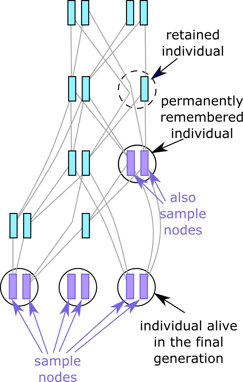
Fig. 7 Individuals not alive in the last generation may still be present in the tree sequence
if they are either remembered permanently (purple),
or simply retained with permanent=F (dotted circle).#
Permanently remembering individuals#
By default, a call to treeSeqRememberIndividuals() will permanently remember one or
more individuals, by marking their nodes as actual samples: the simulated equivalent of
ancient DNA dug out of permafrost, or stored
in an old collecting tube. This means any tree sequence subsequently recorded will always
contain this individual, its nodes (now marked as samples), and its full ancestry. As
with any other sample nodes, any permanently remembered individuals can be removed from
the tree sequence by Simplification. The result of remembering an
individual in the introductory example is pictured on the right.
Retaining individuals#
Alternatively, you may want to avoid treating historical individuals and their genomes as
actual samples, but temporarily retain them as long as they are still relevant to
reconstructing the genetic ancestry of the sample nodes. This can save some computational
burden, as not only will nodes and individuals be removed once they are no longer
ancestral, but also the full ancestry of the retained individuals does not need to be
kept. You can retain individuals in this way by using
treeSeqRememberIndividuals(..., permanent=F).
Since a retained individual’s nodes are not marked as samples, they are subject to the normal removal process, and it is possible to end up with an individual containing only one genome, as shown in the diagram. However, as soon as both nodes of a retained individual have been lost, the individual itself is deleted too.
Note that by default, nodes are only kept if they mark a coalescent point (MRCA or branch
point) in one or more of the trees in a tree sequence. This can be changed by
initialising tree sequence recording in SLiM using
treeSeqInitialize(retainCoalescentOnly=F). SLiM will then
preserve all retained individuals while they remain in the genealogy, even if their nodes
are not coalescent points in a tree (so-called “unary nodes”). Similarly, if you later
decide to reduce the number of samples via Simplification,
retained individuals will be kept only if they are still MRCAs in the ancestry of the
selected samples. To preserve them even if their nodes are not coalescent points, you
can specify ts.simplify(selected_samples, keep_unary_in_individuals=True).
Todo
Add SLiM code which includes retaining and remembering, and perhaps some python code to show them.
Remembering everyone#
Although not needed to reconstruct full genomic history, it is perfectly possible to
apply treeSeqRememberIndividuals() to every individual in every generation of a
simulation (i.e. everyone who has ever lived). If you simply mark everyone for temporary
retention, it should not increase the memory burden of your simulation much: most
individuals will be removed as the simulation progresses, since they will not contain
coalescent nodes. However, if you use treeSeqInitialize(retainCoalescentOnly=F),
the number of individuals in the resulting tree sequence is likely to become very large,
and the efficiencies provided by tree sequence recording will be substantially reduced.
Indeed in this case, retaining will be much the same as permanently remembering everyone
who has ever lived. Nevertheless, if you are willing to sacrifice enough computer memory,
either of these is (perhaps surprisingly) possible, even for medium-sized simulations.
Individual flags#
We have seen that an individual can appear in the tree sequence because it was
Remembered, Retained, or alive at the end of the simulation (note these
are not mutually exclusive). The Individual.flags value stores this information.
For example, to count up the different individual types, we could do this:
Todo
Update this code with the simulation above so that we have some remembered and retained individuals present
indiv_types = {"remembered" : 0,
              "retained" : 0,
              "alive" : 0}
for ind in ts.individuals():
  if ind.flags & pyslim.INDIVIDUAL_REMEMBERED:
     indiv_types['remembered'] += 1
  if ind.flags & pyslim.INDIVIDUAL_RETAINED:
     indiv_types['retained'] += 1
  if ind.flags & pyslim.INDIVIDUAL_ALIVE:
     indiv_types['alive'] += 1

for k in indiv_types:
  print(f"Number of individuals that are {k}: {indiv_types[k]}")
Number of individuals that are remembered: 0
Number of individuals that are retained: 0
Number of individuals that are alive: 2023
Note
In previous versions of SLiM/pyslim, the first generation of individuals were
kept in the tree sequence, to allow Recapitation. With the
addition of the keep_input_roots=True option to the
Simplification process, this is no longer necessary,
so these are no longer present, unless you specifically Remember them.
Generating intial diversity with msprime#
Suppose now that we’d like to start a SLiM simulation with the result of a coalescent simulation. For instance, we might want to do this instead of recapitating if we wanted to use msprime to generate genetic diversity that would then be selected on during the SLiM simulation. To do this, we’ll:
simulate a tree sequence with msprime,
add SLiM information to the nodes and individuals,
add SLiM mutations, and
write it out to a
.treesfile.
First, we’ll (1) run a simulation of 1 Mb of genome sampled in 200 diploids
in a population of 1000 diploids,
and (2) use the annotate() function to add default SLiM metadata to the result:
demog = msprime.Demography()
demog.add_population(initial_size=1000)
ts = msprime.sim_ancestry(
            samples=200,
            demography=demog,
            recombination_rate=1e-8,
            sequence_length=1e6,
            random_seed=5)
ts = pyslim.annotate(ts, model_type="nonWF", tick=1)
assert ts.num_individuals == 200
assert ts.num_samples == 400
We have set tick to 1;
this means that as soon as we load the tree sequence into SLiM,
SLiM will set the current time counter to 1.
(If we set tick to 100, then any script blocks scheduled to happen before 100
would not execute after loading the tree sequence.)
We now have 200 diploids (so, 400 sampled nodes). Here’s individual 199, which hsa SLiM metadata:
ind = ts.individual(199)
print(ind)
Individual(id=199, flags=65536, location=array([0., 0., 0.]), parents=array([], dtype=int32), nodes=array([398, 399], dtype=int32), metadata={
    'pedigree_id': 199,
    'pedigree_p1': -1,
    'pedigree_p2': -1,
    'age': 0,
    'subpopulation': 0,
    'sex': -1,
    'flags': 0
   })
Looking at the metadata above, we see the default values are age=0
hermaphrodites (sex=-1), for instance.
Now let’s add SLiM mutations.
These will be neutral, as msprime.sim_mutations()
doesn’t have the ability to dynamically modify the selection coefficients
stored in the mutation metadata.
To modify the mutations to be under selection,
see Vignette: Starting with diversity generated by coalescent simulation.
ts = msprime.sim_mutations(
                ts, rate=1e-8,
                model=msprime.SLiMMutationModel(type=0),
                random_seed=9
)
Now the mutations have SLiM metadata. For instance, here’s the first mutation:
ts.mutation(0)
Mutation(id=0, site=0, node=88, derived_state='0', parent=-1, metadata={
    'mutation_list': [{
        'mutation_type': 0,
        'selection_coeff': 0.0,
        'subpopulation': -1,
        'slim_time': -42,
        'nucleotide': -1
       }]
   },
time=43.9737541056882, edge=876)
Finally, we write this out to a file that can be loaded in to SLiM:
ts.dump("initialize_nonWF.trees")
Here’s a minimal SLiM script that reads in the tree sequence file and runs it for a bit longer.
initialize()
{
   initializeSLiMModelType("nonWF");
   initializeTreeSeq();
   initializeMutationRate(1e-8);
   initializeMutationType("m0", 0.5, "f", 0.0);
   initializeGenomicElementType("g1", m0, 1.0);
   initializeGenomicElement(g1, 0, 1e6-1);
   initializeRecombinationRate(1e-8);
   defineConstant("K", 1000);
}

reproduction(p1) {
   subpop.addCrossed(individual,
                     subpop.sampleIndividuals(1));
}

1 early() {
   sim.readFromPopulationFile("initialize_nonWF.trees");
   catn("Loaded " + length(sim.subpopulations)
        + " populations from a file; now in generation " + sim.cycle);
   catn("Population sizes: " + paste(sim.subpopulations.individualCount));
}

2: early() {
   p0.fitnessScaling = K / p0.individualCount;
}

10 early() {
   sim.treeSeqOutput("nonWF_restart.trees");
   catn("Done.");
   sim.simulationFinished();
}
%%bash
slim -s 123 neutral_restart.slim
A more in-depth example is provided at Vignette: Starting with diversity generated by coalescent simulation. See the SLiM manual for more about this operation.
Nucleotide-based models#
By default, annotate() produces standard SLiM mutations, not “nucleotide-based” mutations.
To demonstrate how to further adjust the starting state of the simulation,
we’ll further adjust the tree sequence ts from the previous section
to add in information about nucleotides.
First, we need to set the nucleotide_based property in top-level metadata.
To do this, there are two possibly unfamiliar things:
first, we need to modify the underlying tskit.TableCollection
(since tree sequences are immutable);
and second, we have to extract the metadata, modify it, and put it back in
(modifying it in-place will silently do nothing):
tables = ts.dump_tables()
md = tables.metadata
md['SLiM']['nucleotide_based'] = True
tables.metadata = md
ts = tables.tree_sequence()
Next, we need to generate a reference sequence
and nucleotides for each mutation.
This is easy with generate_nucleotides():
ts = pyslim.generate_nucleotides(ts)
ts.dump("initialize_nonWF_nuc.trees")
ts.reference_sequence.data[:20]
'AGAGGTGCCTACTTAGGTGT'
Now, mutations have a nucleotide property in metadata that is not -1:
m = ts.mutation(0)
print(m)
Mutation(id=0, site=0, node=88, derived_state='0', parent=-1, metadata={
    'mutation_list': [{
        'mutation_type': 0,
        'selection_coeff': 0.0,
        'subpopulation': -1,
        'slim_time': -42,
        'nucleotide': 3
       }]
   },
time=43.9737541056882, edge=876)
We can see which nucleotide is the derived state produced by each mutation
by indexing the NUCLEOTIDES object:
for k in range(3):
    m = ts.mutation(k)
    print(f"Mutation {k}: position {ts.site(m.site).position}, time {m.time}")
    for ml in m.metadata['mutation_list']:
        print(f"  nucleotide: {pyslim.NUCLEOTIDES[ml['nucleotide']]}")
Mutation 0: position 6682.0, time 43.9737541056882
  nucleotide: T
Mutation 1: position 8929.0, time 2190.6441703202377
  nucleotide: T
Mutation 2: position 10606.0, time 23.739744183695958
  nucleotide: T
Here’s a script minimally modified from the above to be nucleotide-based:
initialize()
{
   initializeSLiMModelType("nonWF");
   initializeTreeSeq();
   initializeMutationRate(1e-8);
   initializeMutationType("m0", 0.5, "f", 0.0);
   initializeGenomicElementType("g1", m0, 1.0);
   initializeGenomicElement(g1, 0, 1e6-1);
   initializeRecombinationRate(1e-8);
   defineConstant("K", 1000);
}

reproduction(p1) {
   subpop.addCrossed(individual,
                     subpop.sampleIndividuals(1));
}

1 early() {
   sim.readFromPopulationFile("initialize_nonWF.trees");
   catn("Loaded " + length(sim.subpopulations)
        + " populations from a file; now in generation " + sim.cycle);
   catn("Population sizes: " + paste(sim.subpopulations.individualCount));
}

2: early() {
   p0.fitnessScaling = K / p0.individualCount;
}

10 early() {
   sim.treeSeqOutput("nonWF_restart.trees");
   catn("Done.");
   sim.simulationFinished();
}
%%bash
slim -s 123 neutral_nucleotide_restart.slim
Extracting information about selected mutations#
Here is a simple SLiM simulation with two types of mutation:
m1 are deleterious, and m2 are beneficial.
Let’s see how to extract information about these mutations.
initialize()
{
   initializeSLiMModelType("WF");
   initializeTreeSeq();
   initializeMutationRate(1e-6);
   initializeMutationType("m1", 0.5, "e", -0.1);
   initializeMutationType("m2", 0.5, "e", 0.5);
   initializeGenomicElementType("g1", c(m1, m2), c(0.9, 0.1));
   initializeGenomicElement(g1, 0, 1e6-1);
   initializeRecombinationRate(1e-8);
}

1 early() {
   sim.addSubpop("p1", 1000);
}

1000 early() {
   sim.treeSeqOutput("selection.trees");
}
%%bash
slim -s 23 selection.slim
First, let’s see how many mutations there are:
ts = tskit.load("selection.trees")
print(f"Number of sites: {ts.num_sites}\n"
      f"Number of mutations: {ts.num_mutations}")
Number of sites: 6020
Number of mutations: 6044
Note that there are more mutations than sites; that’s because some sites (looks like 24 of them) have multiple mutations. The information about the mutation is put in the mutation’s metadata. Here’s the first mutation:
m = ts.mutation(0)
print(m)
Mutation(id=0, site=0, node=13, derived_state='1653896', parent=-1, metadata={
    'mutation_list': [{
        'mutation_type': 2,
        'selection_coeff': 1.5596729516983032,
        'subpopulation': 1,
        'slim_time': 827,
        'nucleotide': -1
       }]
   },
time=172.0, edge=3100)
Here, m.site tells us the ID of the site on the genome that the mutation occurred at,
and we can pull up information about that with the ts.site( ) method:
ts.site(m.site)
Site(id=0, position=54.0, ancestral_state='', mutations=[Mutation(id=0, site=0, node=13, derived_state='1653896', parent=-1, metadata={
    'mutation_list': [{
        'mutation_type': 2,
        'selection_coeff': 1.5596729516983032,
        'subpopulation': 1,
        'slim_time': 827,
        'nucleotide': -1
       }]
   },
time=172.0, edge=3100)], metadata=b'')
This mutation occurred at position 54 along the genome (from site.position)
which previously had no mutations (since site.ancestral_state is the empty string, '')
and was given SLiM mutation ID 1653896 (m.derived_state).
The metadata (m.metadata, a dict) tells us that
the mutation has selection coefficient 1.5597 and occurred in population 1 in generation 827,
which was 172 generations ago.
This is not a nucleotide model, so the nucleotide entry is -1.
Note that m.time and m.metadata['mutation_list'][0]['slim_time'] are in this case redundant:
they contain the same information, but the first is in tskit time
(i.e., number of steps before the tree sequence was written out)
and the second is using SLiM’s internal “tick” counter.
Also note that the mutation’s metadata is a list of metadata entries.
That’s because of SLiM’s mutation stacking feature.
We know that some sites have more than one mutation,
so to get an example let’s pull out one such mutation.
In this case,
m.metadata['mutation_list'] is a list of length one,
so the mutation was not stacked on top of previous ones.
Let’s pull out a mutation that was stacked on top of another one:
for m in ts.mutations():
  if m.parent != tskit.NULL:
     break

print(m)
print(ts.mutation(m.parent))
Mutation(id=1020, site=1017, node=1597, derived_state='1998096,547531', parent=1019, metadata={
    'mutation_list': [{
        'mutation_type': 1,
        'selection_coeff': -0.0032227179035544395,
        'subpopulation': 1,
        'slim_time': 999,
        'nucleotide': -1
       },
    {
     'mutation_type': 2,
     'selection_coeff': 0.3085740804672241,
     'subpopulation': 1,
     'slim_time': 274,
     'nucleotide': -1
    }]
   },
time=0.0, edge=1213)
Mutation(id=1019, site=1017, node=13, derived_state='547531', parent=-1, metadata={
    'mutation_list': [{
        'mutation_type': 2,
        'selection_coeff': 0.3085740804672241,
        'subpopulation': 1,
        'slim_time': 274,
        'nucleotide': -1
       }]
   },
time=725.0, edge=3100)
This mutation (which is ts.mutation(1020) in the tree sequence)
was the result of SLiM adding a new mutation of type m1 and selection coefficient -0.0032
on top of an existing mutation, also of type m1 and with selection coefficient 0.3086.
This happened at generation 999 (i.e., at tskit time 0.0 time units ago),
and the older mutation occurred at generation 274 (at tskit time 725 time units ago).
The older mutation has SLiM mutation ID 547531,
and the newer mutation had SLiM mutation ID 1998096,
so the resulting “derived state” is '1998096,547531'.
Now that we understand how SLiM mutations are stored in a tree sequence,
let’s look at the allele frequencies.
The allele frequency spectrum for all mutations can be obtained using the
tskit.TreeSequence.allele_frequency_spectrum() method,
shown here for a sample of size 10 to make the output easy to see:
samps = np.random.choice(ts.samples(), 10, replace=False)
afs = ts.allele_frequency_spectrum([samps], span_normalise=False, polarised=True)
print(afs.astype('int'))
[4173 91 6 19 438 1 493 20 0 0 2]
(The span_normalise=False argument gives us counts rather than a density per unit length.)
This shows us that there are 4169 alleles that are found among the tree sequence’s samples
that are not present in any of our 10 samples, 96 that are present in just one, etcetera.
The surprisingly large number that are near 50% frequency are perhaps positively selected
and on their way to fixation: we can check if that’s true next.
You may have noticed that the sum of the allele frequency spectrum is 5243,
which is not obviously related to the number of mutations (6044) or the number of sites (6020).
That’s because each derived allele that is inherited by some but not all of the samples
in the tree sequence is counted in the polarised allele frequency spectrum:
Fixed mutations, or mutations that were entirely “overwritten” by subsequent mutations,
do not contribute.
Here’s how we can check this:
afs_total = 0
for v in ts.variants():
    if len(set(v.genotypes)) > 1:
        afs_total += len(set(v.genotypes) - set([0]))
print(afs_total)
5243
At time of writing, we don’t have a built-in allele_frequency method,
so we’ll use the following snippet:
def allele_counts(ts, sample_sets=None):
   if sample_sets is None:
      sample_sets = [ts.samples()]
   def f(x):
      return x
   return ts.sample_count_stat(sample_sets, f, len(sample_sets),
              span_normalise=False, windows='sites',
              polarised=True, mode='site', strict=False)
This will return an array of counts, one for each site in the tree sequence,
giving the number of all nonancestral alleles at that site found in the sample set
(so, lumping together any of the various derived alleles we were looking at above).
Then, we’ll separate out the counts in this array to get the derived frequency spectra
separately for sites with (a) only m1 mutations, (b) only m2 mutations,
and (c) both (for completeness, if there are any).
First, we need to know which site has which of these three mutation types (m1, m2, or both):
mut_type = np.zeros(ts.num_sites)
for j, s in enumerate(ts.sites()):
  mt = []
  for m in s.mutations:
     for md in m.metadata["mutation_list"]:
        mt.append(md["mutation_type"])
  if len(set(mt)) > 1:
     mut_type[j] = 3
  else:
     mut_type[j] = mt[0]
Now, we compute the frequency spectrum, and aggregate it
to produce the allele frequency spectrum separately by mutation type.
We’ll use the function np.bincount to do this efficiently:
freqs = allele_counts(ts, [samps])
# convert the n x 1 array of floats to a vector of integers
freqs = freqs.flatten().astype(int)
mut_afs = np.zeros((len(samps)+1, 3), dtype='int64')
for k in range(3):
  mut_afs[:, k] = np.bincount(freqs[mut_type == k+1], minlength=len(samps) + 1)

print(mut_afs)
[[3663  484    4]
 [  72   19    0]
 [   4    2    0]
 [  12    7    0]
 [ 251  185    1]
 [   0    1    0]
 [ 285  207    0]
 [  11    9    0]
 [   0    0    0]
 [   0    0    0]
 [ 383  418    2]]
The first column gives the AFS among these 10 samples for the deleterious alleles, the second for the beneficial mutations; the third column for the seven sites that had both types of mutation. Interestingly, there are similar numbers of both types of mutation at intermediate frequency: perhaps because beneficial mutations are sweeping linked deleterious alleles along with them. Many fewer benefical alleles are at low frequency: 3,666 deleterious alleles are not found in our sample of 10 genomes, while only 486 beneficial alleles are.
Finally, let’s pull out information on the allele with the largest selection coefficient.
sel_coeffs = np.array([
        sum(md["selection_coeff"] for md in m.metadata["mutation_list"])
        for m in ts.mutations()
])
which_max = np.argmax(sel_coeffs)
m = ts.mutation(which_max)
ts.site(m.site)
Site(id=2514, position=450121.0, ancestral_state='', mutations=[Mutation(id=2522, site=2514, node=14, derived_state='1616148', parent=-1, metadata={
    'mutation_list': [{
        'mutation_type': 2,
        'selection_coeff': 4.935262680053711,
        'subpopulation': 1,
        'slim_time': 808,
        'nucleotide': -1
       }]
   },
time=191.0, edge=3099)], metadata=b'')
This allele had a whopping selection coefficient of 4.94 and appeared about halfway through the simulation. Let’s find its frequency in the full population:
full_freqs = allele_counts(ts)
print(f"The allele is found in {full_freqs[m.site][0]} copies\n"
      f"out of {ts.num_nodes} genomes.")
The allele is found in 2000.0 copies
out of 3024 genomes.
The allele is above 50% in the population, so it is probably on its way to fixation.
Using its SLiM ID (which is shown in its derived state, 1616148),
we could reload the tree sequence into SLiM,
restart the simulation, and use its ID to track its subsequent progression.
Possibly important technical notes#
Also known as “gotchas”.
If you use msprime to simulate a tree sequence, and then use that to initialize a SLiM simulation, you have to specify the same sequence length in both: as in the examples above, the
sequence_lengthargument tomsprime.sim_ancestry()should be equal to the SLiM sequence length plus 1.0 (e.g., if the base positions in SLiM are 0 to 99, then there are 100 bases in all, so the sequence length should be 100).Make sure to distinguish individuals and nodes!
tskit“nodes” correspond to SLiM “genomes”. Individuals in SLiM are diploid, so normally, each has two nodes (but retained individuals may have nodes removed by simplification: see below).As described above, the Individual table contains entries for
the currently alive individuals,
any individuals that have been permanently remembered with
treeSeqRememberIndividuals(), andany individuals that have been temporarily retained with
treeSeqRememberIndividuals(permanent=F). Importantly, the nodes in these individuals are not marked as sample nodes, so they can be lost during simplification. This means that a retained individual may only have one node (but if both nodes are lost due to simplification, the individual is removed too, and will not appear in the Individual table).
SLiM requires that the two nodes corresponding to the haplosomes of each individual are adjacent in the node table, and are sorted by haplosome ID. SLiM always writes out tree sequences like this, but it is possible to make tree sequences in python that are leval otherwise but don’t satisfy this requirement.